Category: White Papers

Risk Matters
We founded QSV in 2016 to answer the question “how would we want our personal assets to be managed?” With more than twenty-five years of managing client accounts together, we had a philosophy and process in place and knew we could continue to learn and enhance how we invest. A meaningful pillar in our mission statement is to provide a “smoother ride” or the ability for clients to sleep soundly each night without the drama or volatility that some investment styles may deliver. We also founded our business with the belief that attention to risk and setting expectations for clients on how and when we would perform is paramount. QSV’s strategies will not outperform passive benchmarks or our peers in every market environment, but will, we believe, deliver strong risk-adjusted returns and outperformance over full market cycles. Our record to date has proven that to be true.
MEASURING UP (DOWN?)
Tools to evaluate QSV’s performance since the inception of our products include measuring the downside participation that QSV has captured. The downside capture ratio measures how much of the index’s losses a portfolio captures when the market is declining and is calculated by dividing the fund’s returns by the returns of the index during periods when the index is down. In the trailing five years, QSV Mid Cap has delivered downside participation that ranks in the lowest quintile of the Morningstar mid-cap value peer group (rankings sorted from 1st to 100th percentile (with 1st being the highest downside capture to lowest / most favorable in the 100th percentile).
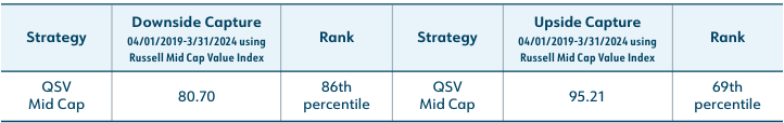
While we strive to improve further on these results, they do reflect well on another pillar of QSV’s mission: to deliver lower drawdowns in challenging markets. Standard deviation of returns is a commonly used measure of volatility to compare an investment portfolio with its benchmark or peers and gives investors a sense of the return “swings” they will endure with a particular portfolio. Here, too, QSV Mid Cap compares favorably with its peers, and ranks in the 86th percentile (with the 100th percentile representing the lowest standard deviation) relative to the Morningstar mid cap value peers. Beta is another tool used to assess the risk of a portfolio. While it is thought that the return potential of a lower beta portfolio is below its benchmark, QSV believes otherwise. In our whitepaper, The Myth of High Beta, QSV questions the long-held belief that higher risk, high beta stocks deliver the highest returns and presents studies that show how the “low volatility anomaly” creates opportunities to beat the market and create long term wealth. QSV Mid Cap has a beta since inception of .73 that ranks in the 90th percentile (with the 100th percentile representing the lowest beta) of the Morningstar Mid Cap Value peer group.
“The lower volatility that QSV has delivered does, we believe, provide the “sleep at night” comfort that many seek.”
QSV MID CAP PERFORMANCE
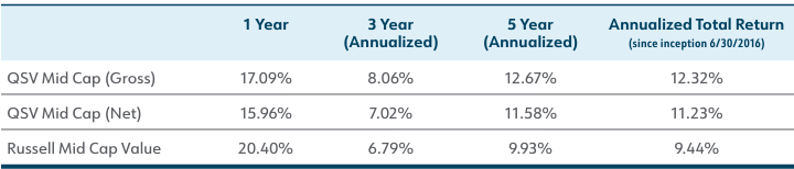
These statistics and their relative ranking are important but are only part of the picture. Returns relative to our benchmark matter to our investors, as well, and QSV has delivered outperformance from its inception through March 31, 2024, fulfilling another of our goals.
Based on this performance, one final statistic and ranking to consider is the Sharpe ratio for QSV Mid Cap. The Sharpe ratio divides a portfolio’s returns in excess of a risk-free rate by its standard deviation of returns to assess its risk-adjusted performance. QSV’s since-inception information ratio of .77 ranks in the 9th percentile (where the 1st percentile is the highest Sharpe ratio) of the Morningstar Mid Cap Value peer group, underscoring the risk-adjusted performance we have delivered for our clients.
WHERE DOES QSV FIT?
We believe that the QSV Small Cap, Mid Cap and Select strategies are great core holdings for clients seeking solutions that will permit them to participate in rising markets while protecting in falling markets, resulting in outperformance relative to passive benchmarks over the long term. The lower volatility that QSV has delivered does, we believe, provide the “sleep at night” comfort that many seek. Choices abound and many clients also wish to have small and mid-cap options in their portfolios that may outperform when QSV lags. This typically happens in times such as rapidly rising markets following recessions and periods of stimulative policies, such as we experienced following the COVID pandemic. QSV has been paired by such clients with deep value managers and high-beta growth managers, where, in both cases, our strategies have offset the periods of underperformance by the other and QSV’s portfolios have dampened the overall risk in the clients’ portfolios.
WHERE ARE WE NOW?
In both Q4 2023 and the first quarter of 2024, QSV noted that we felt much of the potential returns for 2024 had been pulled forward in the performance enjoyed in 2023. Markets got ahead of themselves as investors anticipated waning inflation, multiple interest rate cuts by the Federal Reserve, persistent corporate earnings and continued economic growth. Investors awakened in April to the possibility that these expectations may not come true and their change of heart resulted in volatility and a drop in equity markets. While the markets began 2024 with 150 basis points of rate cuts priced in, valuations currently have seventy-five basis points priced in – what the Federal Reserve had communicated in late 2023 and to which investors failed to pay heed until this recent valuation correction.
We believe that mid-cap stocks are attractive for long-term investors, with valuations relative to large capitalization stocks not seen since the late 1990s. The protracted outperformance of large cap stocks has led to underinvestment in small and mid-cap companies; while mid-caps represented 19.7% of the Russell 3000 Index at year-end, the average investor had only a 10.2% allocation, according to Morningstar. With current economic and geopolitical uncertainties, investors should keenly focus on active management and the ownership of quality businesses to build durable portfolios that can withstand the volatility that may continue. A focus on companies that have strong balance sheets and cash flows in today’s environment is critical.
About QSV Equity Investors
QSV Equity Investors, LLC (formerly Ballast Equity Management, LLC) is an employee-owned asset management firm that invests alongside its clients in high conviction portfolios of quality small and mid-capitalization businesses. QSV manages these portfolios of publicly traded companies for individuals, family offices, and institutions. Based in Naperville, Illinois, QSV was founded in 2016 by Jeff Kautz and Randy Hughes, investment professionals who previously held senior roles at Janus Henderson subsidiary Perkins Investment Management and have invested together for 25 years. For more details on the specific performance and characteristics of QSV’s strategies, including a fully GIPS compliant presentation, please contact Dave Mertens at dmertens@qsvequity.com.
Disclaimer:
This information is provided solely for informational purposes. Full holdings for the QSV Mid Cap strategy and additional information are available by request at customerservice@qsvequity.com. Morningstar Rankings are relative to the Morningstar Mid Cap Value separate account peer group as of March 31, 2024. Returns are for Mid Cap composite of QSV Equity Investors. Gross returns are calculated net of trading fees. Net returns are calculated net of trading fees and net of the firm’s management fee. All dividends are assumed to be reinvested. The returns of the QSV Mid Cap strategy are compared to the historical performance of the Russell Mid Cap Indices as they are a widely used benchmarks for mid capitalization securities. An investment with QSV Equity Investors should not be construed as an investment in a program that seeks to replicate, or correlate with, these indices. Market conditions vary between the QSV products and these indices. Furthermore, these indices do not include any
transaction costs, management fees and other expenses, as do QSV products. Lastly, QSV may invest in securities and positions that are not included in these indices.
No client or potential client should assume that any information presented should be construed as personalized investment advice. Personalized investment advice can only be rendered after engagement of the firm for services, execution of the required documentation, and receipt of required disclosures. Investing carries the risk of loss. QSV Equity Investors, LLC claims compliance with the Global Investment Performance Standards (GIPS®). GIPS® is a registered trademark of the CFA Institute. The CFA Institute does not endorse or promote this organization, nor does it warrant the accuracy or quality of the content contained herein. To view a GIPS report, please visit qsvequity.com. QSV Equity Investors, LLC is a registered investment advisor. For additional information about the firm and its professionals please visit the SEC’s website at adviserinfo.sec.gov.
The Trouble with Point Estimates
The Trouble with Point Estimates
QSV_The Trouble with Point Estimates
NEW BRAND. SAME PEOPLE, PHILOSOPHY AND PROCESS.
The Ballast Equity Management team has worked together for over 25 years, refining our investment philosophy and process, and improving our craft. Our skillset is in researching, valuing, and building portfolios of small and mid-cap stocks and decidedly not in marketing or branding, thus we find ourselves with a corporate name, Ballast Equity Management, which is quite like that of another, peer, firm. As a result, we are rebranding our firm to QSV Equity Investors. QSV stands for the Quality, Stability and Value that we continually seek to deliver to our clients with each decision we make. Our people, philosophy and process will not change, only our name will.
THE TROUBLE WITH POINT ESTIMATES
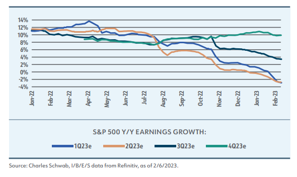
After an era of low interest rates, globalization and low inflation, investors were hit in 2022 with the reality of a new regime, one marked by higher interest rates, inflation, and higher volatility. This new regime has percolated its way into corporate earnings with negative earnings surprises notable in the Communication Services, Information Technology, and Consumer Discretionary sectors. Where earnings for the market go in the near term is difficult to predict, but consensus is that these declines are likely to continue into the next quarter and, we believe, the consensus view may be too rosy for the balance of 2023. At QSV, we worry about the “E” in P/E and feel the game has gotten more challenging for investors seeking to make quick decisions based on the point estimates often used in valuing stocks.
ALL VALUATION TOOLS ARE NOT EQUAL
Point estimates, or market multiples, are widely used by investors and Price to Earnings is the most often used tool for valuing equities. P/E is simple to use, requiring just two inputs. The trailing 12-month price-to-earnings multiple, for example, divides a stock’s current share price by the last year’s earnings per share. The simplicity of this calculation also speaks to its shortcomings– multiples tend only to provide high-level snapshots of valuation at a point in time. These limitations can misguide investors; a P/E may appear low because the company is at peak earnings. Or, without considering what may happen to the “E,” or earnings, in such a simple equation, investors often can step into value traps – stocks that are cheap for good reason – when relying on multiples. Though investors can gain more insight by looking at a company’s P/E multiple over many years or by comparing it to the market and other companies in the same industry, there is another critical drawback; valuation multiples still do not account for cash and debt on the company’s balance sheet. More importantly, they do not account for a company’s potential growth or its risk profile. Because of such limitations, we at QSV may use these ratios in our initial screening process, but we rely on a more robust model to derive our ultimate intrinsic value estimates.
QSV relies on a proprietary, and more sophisticated, valuation model to identify winning companies. Our Economic Profits model enables us to take a closer look at what a prospective firm has going on under the hood. Economic Profits and Discounted Cash Flow (DCF) models are similar and should arrive at the same intrinsic value for a company. However, we believe the Economic Profits model, which considers both the cost of debt, as DCF does, as well as the cost of equity, provides additional insight. By studying the firm’s capital structure and allocation decisions, such as its debt levels, tax rates, share repurchases and dividend payouts, QSV can assess whether management’s capital allocation decisions are creating or destroying value, making this model a more comprehensive tool for valuing a firm’s stock.
FUNDAMENTALS IN FOCUS
Before the valuation process begins, QSV conducts thorough quantitative and qualitative analysis to seek out businesses with competitive “moats.” We believe that business performance, including high margins, reverts to the mean over time, but we also believe that competitive advantages enable companies to maintain higher than average performance for longer periods of time. High quality companies tend to remain high quality companies. This persistence helps us value the stocks of these companies with a higher degree of conviction.
Easy money and rising markets created wealth and nascent investment success in areas that would never have occurred to Ben Graham or Warren Buffett at the beginning of the post-financial crisis era. Passive investing made a great percentage of active managers look passé. Meme stocks made work from home traders temporarily wealthy. Thematic ETFs focused on these meme stocks, on our politicians’ personal trading, and on other “disruptive” ideas capitalized on investors’ optimism, yet often went from hot to cold with startling speed. In the current environment of greater uncertainty, higher borrowing costs, and earnings headwinds, we believe investors would be prudent to emphasize active management in quality businesses, those with durable competitive advantages, strong balance sheets and strong and growing free cash flows.
About QSV Equity Investors
QSV Equity Investors (formerly Ballast Equity Management) is an employee-owned asset management firm that invests alongside its clients in high conviction portfolios of quality small and mid-capitalization businesses. QSV manages these portfolios of publicly traded companies for individuals, family offices and institutions. Based in Oakbrook Terrace, Illinois, QSV was founded in 2016 by Jeff Kautz and Randy Hughes, investment professionals who previously held senior roles at Perkins Investment Management and have invested together for over 20 years. For more details on the specific performance and characteristics of QSV’s strategies, including a fully GIPS compliant presentation, please contact Dave Mertens at dmertens@qsvequity.com.
Lessons Learned in 25 Years of Investing Together
QSV_Lessons Learned in 25 Years
QSV Equity Investors was founded in 2016 as an independent, employee-owned advisory firm by Jeff Kautz and Randy Hughes. Jeff and Randy began investing together twenty-five years ago at Perkins Investment Management, where their boss and mentor, Bob Perkins, first hired Randy in 1995 and then Jeff in 1997. The business and their careers grew. From assisting Bob in the management of a $30 million small cap value fund the late 1990s to responsibilities on multiple value products and over $20 billion in assets by 2016, Jeff became CEO and Chief Investment Officer of the firm and Randy held the roles of Director of Research and Analytics and Equity Analyst. Jeff also served as co-manager of the Janus Henderson Mid Cap Value Fund and the Janus Henderson Value Plus Income Fund.
Twenty-five years into their partnership, Randy and Jeff remain value investors and lessons have been learned over that period. The tools used, and the approach taken to investing clients’ assets have evolved, with the philosophy that investing is a craft where you can learn and get better over time. Seven key lessons, our reflections, and what we believe are the benefits to our clients, follow.
CHEAP IS NOT ENOUGH; QUALITY BOUGHT AT A REASONABLE PRICE ADDS VALUE
Early in their careers at Perkins, Jeff and Randy focused on cheap stocks, using the 52-week lows list as the starting point for their investment process. Subsequent process steps dug into the fundamentals of each company and an assessment of the durability of its business model. As they gained experience, Jeff and Randy gained conviction in the critical importance of quality and the durable competitive advantages that certain companies earned through successful execution. Their conviction was supported by the “smoother ride” that companies with the characteristics of quality, including strong balance sheets, persistent returns on invested capital, strong and growing free cash flows, and lower levels of debt, delivered. Performance of the Russell Defensive Small and Mid-Cap indexes relative to the Russell value indexes supports this over the last fifteen years as shown on the next page.
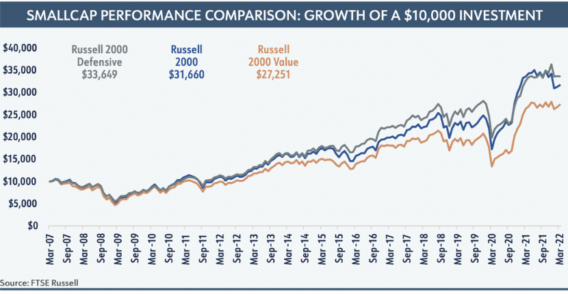
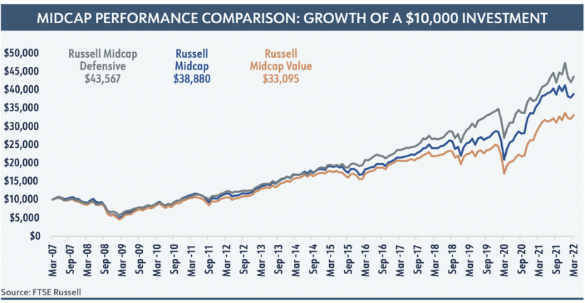
Much like the qualities sought by QSV, the Russell Defensive indexes emphasize stocks that exhibit a combination of high return-on-assets, low debt-to-equity, low earnings variability, and low long- and short-term total return volatility. QSV starts its investment process with a singular focus on quality, using both quantitative and qualitative tools to assess the durability of prospective holdings. This focus is grounded in the understanding that we are owners of each business, not traders in its stock.
ALL VALUATION TOOLS ARE NOT EQUAL
Over the course of our twenty-five years of working together, Jeff and Randy have used many methods of valuation. While some can be more useful than others, they have found that these conventional tools are insufficient to meet the needs of the modern investor.
Valuation multiples are the most widely used measures for valuing equities because they are simple to use. These multiples require only two inputs – an estimate of the firm’s value in the numerator and a measure of some valuation metric in the denominator. For example, the trailing 12-month price-to-earnings multiple simply divides a stock’s current share price by the last year’s earnings per share. The simplicity of this type of value calculation also speaks to its shortcomings – multiples tend only to provide high-level snapshots of valuation at a point in time. These shortcomings can misguide investors; a P/E may appear low because the company is at peak earnings. Or, without considering what may happen to the “E,” or earnings, in such a simple equation, investors often can step into value traps – stocks that are cheap for good reason – when relying on multiples.
Another common method of valuation is the Enterprise Value formula, which is used to represent a business’ book value, or the total cost of acquiring that business today. The cost of acquisition can be calculated by adding the total market value of the company’s equity to the total debt that it carries. The resulting sum is a shorthand (though widely accessible) figure that, like multiples, does little to inform us of a business’ investment-worthiness.
Discounted cash flow analysis provides a more accurate measure of the intrinsic value of a business by considering the present value of the cash flows the company is expected to generate in the future and discounting them to arrive at a current, present value. DCF calculates a company’s intrinsic value based on cash flow projections far into the future, which are discounted back to a present value using a combination of a risk-free rate and an equity risk premium. Predicting cash flows is tricky – they are likely to change in time – but a company is not as likely to try to distort cash flows the way it may do with earnings. And applying this cash flow analysis to more predictable, quality businesses is more prone to good outcomes than when assessing more volatile or cyclical businesses.
We lean on QSV proprietary, and more sophisticated, valuation model to identify winning companies. Our Economic Profits Model enables us to take a closer look at what a prospective firm has going on under the hood. Economic Profits and Cash Flow Models are similar and should arrive at the same intrinsic value for a company. However, we believe the Economic Profits Model, which considers both the cost of debt, as DCF does, as well as the cost of equity, provides additional insight. By studying the firm’s capital structure and allocation decisions, such as its debt levels, tax rates, share repurchases and dividend payouts, QSV can assess whether management’s capital allocation decisions are creating or destroying value, making this model a more comprehensive tool for valuing a firm’s stock.
RISK MEANS DIFFERENT THINGS TO DIFFERENT INVESTORS
Allocators today consider many measures of “risk” when weighing the results of QSV and its peer investors. Statistics including standard deviation of returns, downside deviation, drawdown and tracking error relative to an index are among the tools used and, while helpful, are all backward looking in their measurement, using data that is in the past. QSV considers the fundamentals of each prospective investment (using backward looking data) and then considers the prospects of that business looking forward, concentrating our ownership on what we believe will be the best wealth creating holdings for our clients. As owners of a portfolio of quality businesses and as fiduciaries to our clients, QSV views risk as the permanent loss of capital. Our insistence on quality businesses leads to another benefit, albeit a residual of our process; QSV portfolios consistently have lower standard deviations of returns than their indexes.
INDEXES ARE NECESSARY TOOLS, BUT POOR MASTERS
“What gets measured gets done” is a popular saying used to emphasize the importance of performance measurement in business and the business of investment management is no different. Investment indexes are the industry’s tools to benchmark the results of each portfolio over time and, like popular risk measurement statistics, QSV sees these as a necessary tool for our clients and their advisors. We do not manage portfolios with an eye toward adhering to the sector weights or holdings of the relevant index, however, but build portfolios one business at a time. Relative to value indexes and many of our value peers, this generally results in greater exposures to segments of the economy such as healthcare, technology, and consumer staples businesses, where we find quality businesses that possess durable competitive advantages or “moats.” QSV finds fewer of these businesses and has lower weights relative to the indexes in the energy, materials, and financial sectors. Understandably, this results in performance of the portfolios that may be quite different than the indexes in short term periods. QSV always counsels clients to expect this, but we believe we can deliver performance greater than both the value and core indexes over full market cycles, with less risk.
PATIENCE AND CAREER RISK DO NOT LIVE WELL TOGETHER
Delivering excess performance, or alpha, is challenging and even the most skilled investors will have periods, sometimes extended periods, of underperformance. Clients, their advisors, and, as a result, large, publicly-traded investment houses, routinely measure the results of their portfolios against relatively short one- and three-year periods. This is a reality of the business but creates risks to the employment status of many investment professionals. An independent, employee-owned firm must answer to these same client demands but can structure employment and compensation programs to reflect the longer periods of time that may be needed to demonstrate the merits of an investment strategy. At QSV, we believe the correct way to assess the success of a portfolio manager is over a full market cycle, including both peaks and troughs.
CLIENT FIT IS LIKE MARRIAGE
Just as it is difficult to deliver outperformance in active management, it can be hard for asset owners to hold actively managed portfolios, given the disconnects between managers and their respective indexes and periods of underperformance. Just as in a marriage, humility, patience, time, honesty, trust, and communication are all necessary for a successful relationship between a client and its investment managers. QSV is judicious in setting client expectations early in each relationship. We strive to communicate openly and often, and take ownership of our results, both good and bad. Our intention is to have long, trusting relationships with clients who can invest alongside us and benefit from our work.
CULTURE MATTERS
Culture is critical to the success of a business where the assets – human capital – walk out the door every evening. QSV’s team members have worked in small, independent firms and in large publicly traded businesses. We have learned that maintaining the cultural traits that support delivering results for our clients and retaining motivated employees is best done in an independent, employee-owned firm. Traits we hold as critical are:
- Ownership of our defined, repeatable approach to investing.
- Team members sharing a passion for research, investing and client service.
- An ego-free culture that combines diverse, independent thought with collaborative decision-making.
- An emphasis on investment excellence over asset gathering.
- Employee ownership and a willingness to share ownership with key contributors.
CONCLUSION
Lessons learned are often the result of mistakes made and in twenty-five years of investing together Randy and Jeff have made their share. Admitting to those errors, learning, and making the adjustments necessary to QSV’s investment process over time is what will enable us to add value for our clients going forward. The investment world has changed immensely in twenty-five years, with the availability of more information facilitated by rapidly changing technology, changes in investors’ preferences, and with more competition from active and passively managed investment vehicles. QSV’s emphasis on owning quality businesses that create wealth for clients persists, while our process for finding the best of those companies at compelling valuations continues to be refined. We are reminded of the advice of baseball manager Jimmy Dugan in A League of Their Own: “Of course it’s hard. It’s supposed to be hard. If it were easy, everybody would do it. Hard is what makes it great.” We will continue to do the hard work, learn from our mistakes, and refine our craft as we serve our clients.
“Of course it’s hard. It’s supposed to be hard. If it were easy, everybody would do it. Hard is what makes it great.”
ABOUT QSV EQUITY INVESTORS, LLC
QSV Equity Investors, LLC is an employee-owned asset management firm that invests alongside its clients in high conviction portfolios of quality small and mid-capitalization businesses. QSV manages these portfolios of publicly traded companies for individuals, family offices and institutions. Based in Oakbrook Terrace, Illinois, QSV was founded in 2016 by Jeff Kautz and Randy Hughes, investment professionals who previously held senior roles at Perkins Investment Management and have invested together for over 20 years. For more details on the specific performance and characteristics of QSV’s strategies, including a fully GIPS compliant presentation, please contact Dave Mertens at dmertens@ballastequity.com.

Sustainability Inside
Sustainability Inside
November 2021
The “Intel Inside” advertising program that began in 1991 is thought to be the most powerful cooperative marketing program in history. Intel Corporation successfully aimed its advertising toward consumers, convincing them that Intel chips were the ingredient needed to have a positive personal computing experience. Today, ESG investing is capturing minds and investment dollars, with both individual and institutional investors driving flows toward funds that emphasize environmental, social, and governance issues. According to Morningstar, assets in U.S. sustainable funds totaled more than $330 billion as of September 30, 2021, a 9% increase over the previous quarter and 1.8 times the $183 billion record set one year earlier, in the third quarter of 2020.i QSV Equity Investors does not represent itself as an ESG firm or its investment strategies as ESG focused. QSV does, however, consider ESG factors as part of its investment process and many of its holdings have strong sustainability initiatives in place. Investment considerations begin prior to QSV’s investment and will continue during our ongoing monitoring of portfolio companies. As with every investment decision, QSV takes a company-specific approach and understands that ESG factors vary across industries, geography, and time.
ESG data is readily available from most large corporations, but disclosures have lagged among small-mid cap companies that have lesser resources to devote to disclosure and reporting. This has left investors with an incomplete view of the initiatives and risks that may exist. QSV maintains its focus on these small and mid-capitalization companies, with the belief that its quality-biased, value equity strategies can add alpha for its clients over full market cycles. Based on investor demand, more sustainability disclosures are becoming available from these small to medium cap companies. A survey conducted by White & Case, LLP, while limited in scope, showed that small and mid-cap companies providing sustainability disclosures rose from 35% to 51% in the 2019 to 2020 period.ii Such disclosures permit QSV to supplement the detailed analysis it has historically done to understand each business, its risks, and opportunities more deeply.
ESG and sustainability initiatives within QSV’s holdings
Copart (CPRT) operates the largest global marketplace for salvage vehicles. The company has established wide moats based on its property ownership, permitting vehicle storage, and a global digital marketplace that drives strong auction returns. By definition, its role in the recycling of salvage vehicles, either as drivable cars or reusable parts, lessens the impact on the environment of cars that would otherwise be scrapped. Many of the vehicles sold through Copart’s auction platform are purchased for use in developing countries where affordable transportation is a critical enabler of economic development, agriculture production, education, health care, and well-being. Other important steps taken by the business include operating heavy equipment with the latest and cleanest emissions technology available, maintaining a tire recapping program to limit the effects on the environment of tire manufacturing and waste, and the implementation of operational policies that control fuel burn and idling that have reduced use by over 300,000 gallons per year, significantly reducing generated emissions.
ICON PLC (ICLR) offers late stage outsourcing services to pharmaceutical, biotechnology and medical device companies. Noteworthy is its recent support of Pfizer and BioNTech on their COVID-19 vaccine trial, where the company worked with 153 sites in the US, Europe, South Africa, and Latin America to ensure the recruitment of more than 44,000 trial participants over a four-month period. Also of note is the nature of ICON’s business, where its leadership in the development of new drugs can have a significant impact on patient health and wellbeing. The company established its ESG Committee in 2019 and has established specific goals and objectives aligned with the 2030 United Nations Sustainable Development Goals. Among these are environmental goals to use 100% renewable electricity by 2025, a 20% reduction in kilowatt hours of electricity by 2030 and net zero carbon emissions on Scope 1 & 2 by 2030. ICON has significant diversity and inclusion efforts in place, led by its Inclusion & Belonging Steering Committee. Governance is strong, with eight independent directors out of ten as of December 2020. Following the merger of ICON with PRA, four of the twelve board seats are held by women.
Professional employer organization Insperity, Inc. (NSP) fills a lucrative niche within mid-high income white-collar employers, serving them as they outsource their increasingly complex human resources and benefit services needs. NSP has conservation initiatives to improve its carbon footprint. 463,400 pounds of paper are recycled through NSP’s conservation efforts, equivalent to 3,940 trees saved, 88,000 gallons of oil, 1.62 million gallons of water, and 695 cubic yards landfill space. NSP is highly involved in the community, with 60% of NSP’s employees participating in community activities. NSP also fosters a culture of Diversity, Equity and Inclusion which helps its own employees as well as its clients.
QSV holding LabCorp (LH) chartered an ESG Steering Committee in 2020 that works together with the company’s CEO and Executive Committee. The company has environmental initiatives in place to reduce emissions and optimize energy consumption. These include optimizing its courier vehicle fleet, investing in more energy efficient equipment and LED lighting, and utilizing renewable energy sources. In 2019, the company reduced greenhouse gas emissions by 3.6% while total energy consumption was flat relative to the prior year. Led by its Chief Diversity and Inclusion Officer, social initiatives include adding historically Black colleges to key recruiting schools, putting greater emphasis into developing female leadership and facilitating forums for women to share perspectives with the executive team, and promoting use of employee resource groups. In 2020, 78% of global interns were female and, in the U.S., 32% were underrepresented minorities. LabCorp was one of only 18 companies recognized by the U.S. National Business Group on Health for the Best Employers Excellence and Well-Being Platinum Award. Governance is a critical issue within LabCorp and in QSV’s analysis of the business. Nine out of 10 board members are independent, and five out of 10 board members are female and/or ethnically diverse. Stockholder friendly policies include annual election of directors, annual say-on-pay vote, shareholder right to call special meetings, and no supermajority voting requirement. 77.5% of CEO compensation is performance based and at risk.
For two consecutive years, Watts Water Technologies (WTS) has been named by Newsweek magazine as one of “America’s Most Responsible Companies.” The company is uniquely situated to aid in energy conservation as it provides water and gas products that contribute to energy efficiency and the sustainability of water supplies for commercial and residential uses. The company benefits from a shift to eco-friendly products and is committed to delivering 25% of revenue from smart and connected products by 2023. Watts has reduced its water intensity by 39% since 2019, has reduced 4,000 metric tons of CO2 and avoided 830,000kWh of electricity. Watts is involved in community outreach, such as its Covid-19 relief efforts where it supplied front-line healthcare workers with personal protective equipment, donated laptops and school supplies to students for remote learning and raised over $21.5 million to support 43,000 restaurants across the U.S.
Next Steps
Intel has moved beyond 1991 and the 386 microprocessor. ESG investing and its definitions will also evolve, likely becoming a more meaningful source of new data to supplement traditional investment data. The QSV team also began working together in the 1990s and has refined its process and accountability to clients over that time. Our emphasis on quality businesses, ones that deliver persistent earnings and returns on invested capital supported by durable competitive advantages, has remained steadfast in this period. This focus leads us to companies that are often forerunners in pursuing sustainability initiatives. Management of these companies know that such initiatives may provide pathways to improved business performance that should support attractive returns and risk profiles for investors. QSV will continue to enhance our research, paying careful attention to sustainability initiatives and acknowledging that they offer a valuable addition to the fundamental characteristics our process demands.
About QSV Equity Investors, LLC
QSV Equity Investors, LLC is an employee-owned asset management firm that invests alongside its clients in high conviction portfolios of quality small and mid-capitalization businesses. QSV manages these portfolios of publicly traded companies for individuals, family offices and institutions. Based in Oakbrook Terrace, Illinois, QSV was founded in 2016 by Jeff Kautz and Randy Hughes, investment professionals who previously held senior roles at Perkins Investment Management and have invested together for over 20 years. For more details on the specific performance and characteristics of QSV’s strategies, including a fully GIPS compliant presentation, please contact Dave Mertens at dmertens@ballastequity.com.
_______________________________________________________________
i https://direct.morningstar.com/research/doc/1063673/Global-Sustainable-Fund-Flows-Q3-2021-in-Review
ii A Survey of Sustainability Disclosures by Small and Mid-Cap Companies (harvard.edu)

A Quality Upgrade for Mid Cap Investing
QSV is pleased to celebrate another significant milestone, the fifth anniversary of the firm’s Quality Value Midcap strategy. QSV’s founders, Randy Hughes and Jeff Kautz, have managed U.S. mid cap equity portfolios as a team for more than twenty years and believe this asset class to be the “sweet spot” for investors, one deserving of greater attention and, in many cases, larger allocations.
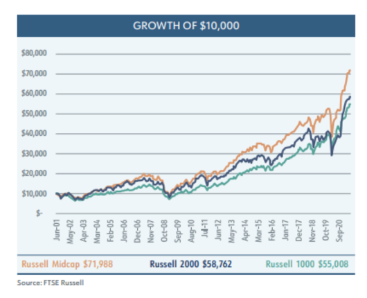
The case for U.S. mid cap stocks has been made before. Relative to large capitalization stocks, mid caps exhibit stronger earnings growth, and offer greater potential returns. Relative to small capitalization stocks, mid caps are more established (reducing the going concern risk), less reliant on having access to capital, less volatile and more liquid. We believe this argument holds merit. Looking at the growth of $10,000 over the previous twenty years, we see that mid cap stocks have outperformed both small cap stocks, represented by the Russell 2000
Index, and large cap stocks, represented by the Russell 1000 Index.
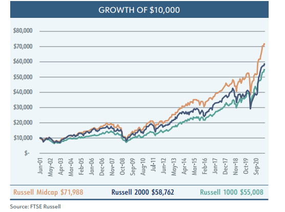

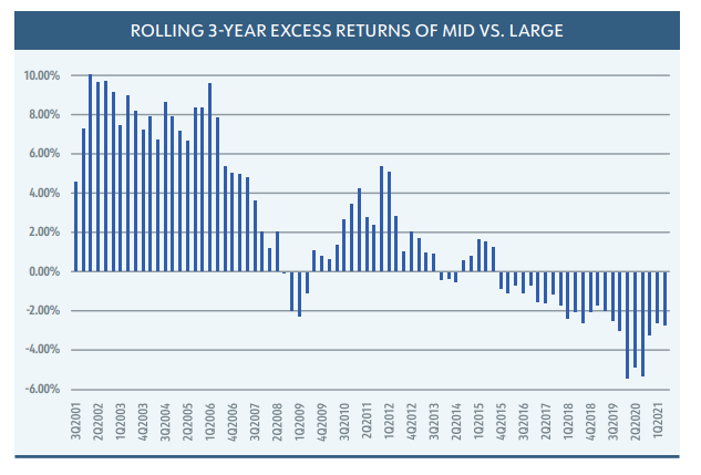
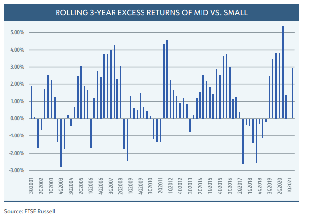
Even if that chart is broken down into periods of rolling three-year returns, we see that mid cap stocks outperform large caps in 63% of those periods and outperform small capitalization stocks in 73% of those three-year periods.

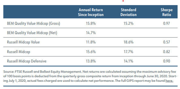
While these numbers alone seem to argue for a greater commitment to mid cap stocks, an even stronger case can be made. By adding a quality overlay to a mid cap strategy, we believe it is possible to structure portfolios that will exhibit 90% upside capture and 70% downside capture. The result being a portfolio that outperforms the market over a full market cycle with less volatility, thereby looking even more appealing on a risk-adjusted basis.
Many investors claim to buy high quality companies. No investor ever admits that they buy low quality companies. At QSV, we have proprietary factor-based scores that we utilize as a starting point to define quality. Companies that exhibit strong returns on invested capital (well in excess of their cost of capital), high free cash flows, high financial flexibility and low capital intensity tend to screen well in our quality rankings. QSV also looks for the presence of a durable competitive advantage, or moat, to help preserve those strong financial characteristics. The combination of these factors is the definition of a high quality company in our investment framework.
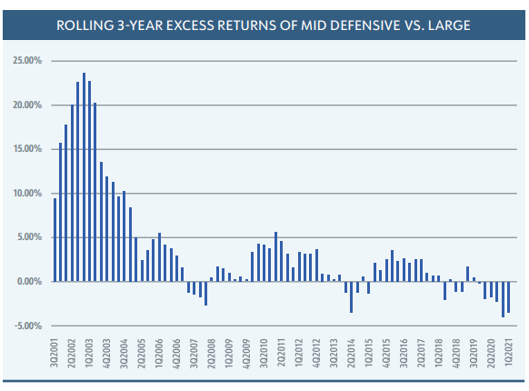
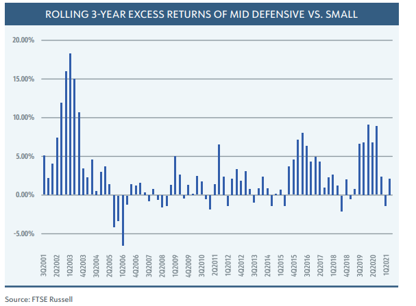
FTSE Russell has done some interesting work with their style-based Stability Indexes, which include a series of defensive and dynamic indices. Russell’s defensive indices utilize a number of the traits we would associate with high quality companies, while their dynamic indices would be what we consider high-beta, lower quality companies. If we look at the same growth of $10,000, what we see is that by adding a quality overlay we can indeed boost the excess return of a portfolio.

Furthermore, by adding a quality overlay, the percentage of rolling three-year periods in which mid cap stocks out-perform increases to 78% relative to large capitalization stocks and to 78% relative to small capitalization stocks.

In an environment where artificially low rates are forcing investors to take on more risk to meet their return objectives, we believe that investors would benefit from exposure to high quality midcap stocks in their portfolios. As we look back on our first five years since launching QSV Equity Investors, we believe we are off to a good start in delivering on our promise to investors. QSV Quality Value Midcap strategy has outperformed its primary benchmark while taking on significantly less risk in our clients’ portfolios. This has led to risk-adjusted returns well in excess of our benchmarks as indicated by the Sharpe Ratio of the QSV Quality Value Midcap strategy.

QSV has worked for over 20 years to refine our process of identifying and investing in high quality companies. Our approach requires patience. There will be periods of underperformance, typically coming out of a recession, which we are experiencing now. We do not believe anyone has the ability to consistently time the markets, and we do not attempt to. We believe the better approach is to take a long-term view toward investing that goes beyond simple quarterly or annual returns and focuses on risk-adjusted returns over a full market cycle that includes both peaks and troughs. In doing so, we are confident in our belief that we can outperform our peers and benchmarks and help our clients achieve their long-term financial goals.

A Valuation Framework for Beating Inflation and Creating Long-Term Wealth
QSV_ A Valuation Framework for Beating Inflation and Creating Long Term Wealth
“It’s far better to buy a wonderful company at a fair price than a fair company at a wonderful price”- Warren Buffett
We often see individual investors get stuck thinking of stocks as short-term trading vehicles. In our opinion, investors who consider themselves owners of companies rather than owners of stocks are more likely to be successful in reaching their goals. As owners, investors should not accept a return on their investment that is less than the risk-free rate plus an equity risk premium. Too often, people invest with long shot hopes of achieving short-term jackpot type returns. They forget the long-term goals of investing – beat inflation and create wealth.
One of the hardest things for investors to do is to separate day-to-day stock price gyrations from the fundamentals of the companies they own. It may help to remember that high quality companies are more likely to generate strong returns on capital regardless of stock market gyrations. In addition, if the economy slows or declines, profits of quality companies should suffer less, which means their stock prices, in theory, should also fall less. Investors (aka owners) of such quality companies should be able to grow their own wealth in line with wealth-creating companies.
Successful investors like Warren Buffet are able to outperform their peers and benchmarks over time precisely because they think long term and differentiate between company fundamentals and stock market volatility. This is why when the market corrects and people ask Mr. Buffet for his opinion, he typically answers, “I have total faith in the U.S. economy.” Other professional investors offer opinions on where stock prices will be the next day, the next month, the next year. Mr. Buffet doesn’t care where his stocks trade on any given day. He understands that day-to-day gyrations don’t affect the long-term fundamentals of the companies he owns. This is why Buffet often acquires entire companies when he truly believes in their long-term fundamentals. This, in effect, takes market volatility out of the equation.
The ideal stock is priced below its intrinsic value and produces high returns on capital, with relatively low levels of risk. Unfortunately, most investors are more likely to buy stocks when they are priced above value, have returns that are reverting to the mean, and carry higher risk than expected. In fact, the market (made up of investors) usually craves high momentum, expensive growth stocks. In the U.S., investors most often favor stocks that are expensive as measured by price-to-earnings or price-to-book ratios. These stocks tend to have very low dividend yields and very high expected growth rates. They also tend to have experienced high price momentum over the previous 12 to 24 months. In our experience, such stocks have not been “ideal” for creating long-term wealth.
So how do investors decide when the price is right? In this paper, we will review pros and cons of some popular valuation frameworks. We will also present the valuation framework we at QSV apply to help investors beat inflation and create long-term wealth.
Popular Valuation Frameworks
Multiple-Based Valuation
Value multiples are by far the most widely used measures for valuing equities, probably because they are very simple to use. Value multiples require only two inputs – an estimate of the firm’s value in the numerator and a measure of some valuation metric in the denominator. In other words, a valuation multiple is simply dividing the price of the company by a factor that is believed to drive value for that company. For example, the trailing 12-month price-to-earnings multiple simply divides a stock’s current share price by the last year’s earnings per share.
Other commonly used valuation multiples are price-to-book value, price-to-cash flow, and price-to-sales. All else being equal, investors would want to pay as little as possible for each unit of earnings, book value or whatever other value measure they choose. These ratios are widely used due to their simplicity, but one disadvantage is that they provide only a snapshot of a company at a given point in time. Though investors can gain more insight by looking at a company’s multiple over many years or by comparing it to the market and other companies in the same industry, there is another critical drawback. Valuation ratios still do not account for cash and debt on the company’s balance sheet. More importantly, they do not account for a company’s potential growth or its risk profile. Because of such limitations, we at QSV Equity may use these ratios in our screening process, but we rely on a more robust model to derive our ultimate intrinsic value estimates.
Enterprise Value
Another measure of a company’s worth is enterprise value, which is the price an acquirer would pay to buy an entire company. Enterprise value represents the worth of a company’s ongoing business. As discussed above, traditional equity multiples like the p/e ratio, price-to-book value, and price-to-cash flow only show the value of shareholders’ claims on the business’s earnings, assets, or cash flows. Multiples of enterprise value, however, reflect the value of all claims on
a business.
Enterprise Value = Market Value of Equity + Net Debt
Enterprise value best represents a company’s “takeover value” – what it would cost to buy the entire company. It’s different from the more commonly quoted measure of company value – market capitalization, which is the cost of buying all of a company’s outstanding shares. If you buy the entire company, you also assume its debt obligations. Furthermore, any cash the company has on its balance sheet can be used to pay down those debt obligations, so we deduct cash from total debt to arrive at a value for net debt. Adding net debt to the market value of outstanding equity gives us a better measure of a company’s fair value.
Consider the following example. Company A and Company B both have market capitalizations of $100 million with $10 million of earnings before interest and taxes (EBITDA). Therefore, both would trade at 10x EBITDA, using a traditional price-to-cash flow multiple.
However, someone who wanted to acquire the entire company would need to consider the firm’s capital structure. If Company A has $20 million in cash and no debt (net CASH of $20 million), while Company B has no cash and $20 million in debt (net DEBT of $20 million), then the enterprise value of Company A is $80 million ($100 + $0 – $20) while Company B is $120 million ($100 + $20 – $0). From an acquirer’s perspective, utilizing the EV/EBITDA framework, Company A would appear cheaper as follows:
Company A = Enterprise Value / EBITDA = $80 million / $10 million = 8X
Company B = Enterprise Value / EBITDA = $120 million / $10 million = 12X
This example demonstrates how important it is to consider capital structure when evaluating company valuations and why we believe multiples of enterprise value are a significant improvement over simple price multiples.
Discounted Cash Flow Model
At the most basic level, a firm’s theoretical value is equal to the present value of its future cash flows. This is called a discounted cash flow (DCF) model. Unlike multiple-based valuation, which is a snapshot of current valuation, DCF models project cash flows many years into the future and then determine what those future cash flows are worth today. This may be a more accurate way to measure valuation, but it takes more time and includes additional projections that may dramatically change the valuation.
Free cash flow (FCF) models are popular because they calculate financial performance as operating cash flow minus capital expenditures, which shows the true cash coming into and going out of a business. A company can appear very profitable on the surface – for example based on earnings per share (EPS) – but actually have a net negative cash flow.
Analyzing cash flow statements from many previous years should provide a clear picture of how healthy a company has been and also provide guidance on how to project cash flows into the future. It is particularly important to note how a company performed during industry downturns or a recession because these indicate whether the company was able to continue generating free cash flow during difficulties.
After determining a company’s free cash flow, it is possible to forecast future free cash flow and develop a discounted free cash flow model using the
following formula:
DCF = [(CF1) / (1 + r)] + [CF2 / (1 + r)2] + … + [CFn/(1+r)n]
CF = Cash Flow
r = Discount Rate (weighted average cost of capital or WACC)
An additional benefit is that DCF models value a firm based on metrics well within management’s control, such as operating profits and capital allocation decisions, rather than arbitrary metrics such as market capitalization and share price that depend on what the market thinks about the company.
The QSV Equity Approach to Measuring Value, Beating Inflation, and Creating Wealth
When we at QSV are deciding whether or not to own a stock, what we really want to determine is if the company is able to create wealth and what will the company be worth well into the future. As we said above, valuing stocks using multiples is helpful for determining what a stock is worth at one point in time. For example, PE multiples are typically based on earnings per share for either the last 12 months, current year or next year. At QSV, we do not plan to trade in and out of stocks, so we rely on a more comprehensive valuation strategy to identify companies that will create long-term wealth in order to help our clients beat inflation while investing for and during retirement.
Companies can create wealth only if they are able to generate a return on invested capital that is greater than the cost of that capital. In the simplest terms, a company must earn more on its money than what it pays to borrow that money.
Example: A company borrows $100 million at a 5% rate of interest and sells 10 million shares to the market at $10 dollars each. The capital invested in the firm is $200 million ($100 million debt + 10 million shares x $10 per share). We already know the debt cost 5%. To make it simple, assume the equity cost 10%, and the company pays no tax on its profits. So, half of the company’s capital costs 5% and the other half costs 10%.
The total cost of capital is: (50% x 5%) + (50% x 10%) or 7.5% per year
This is also known as the Weighted Average Cost of Capital (WACC). In order to create any value, the company must earn at least 7.5% on the capital borrowed from its lenders and investors. All else being equal, if a company earned only 7.5% in perpetuity, investors should never pay more than the original $10 per share of stock because the company is neither creating nor destroying capital. If the rate of return on the invested capital increases above 7.5%, the company’s stock should be worth more because the company is creating wealth. If the rate of return is below 7.5%, the stock should eventually fall below $10 because the company is destroying value by earning less than its cost to borrow.
Company management, employees, and investors want a company’s enterprise value to be as high as possible compared to the capital invested in the company. However, companies that destroy capital may still trade above its invested capital. Either investors believe a particular company will eventually create value or they don’t recognize that the company is not positioned to create wealth over time (even if it appears to be exciting and growing earnings at a fast pace).
For successful long-term investing, we need a valuation framework that helps us identify companies that add value and create wealth over time versus those that destroy capital. We believe Economic Profits does just that and have made it the basis of QSV’s Equity’s valuation framework.
Economic Profits
The Economic Profits Model is an extension of the DCF model discussed above. The two valuation methodologies should yield the exact same result for firm value. The primary difference is that DCF models only take a charge for the debt portion of capital (by subtracting interest expense from operating income), while an Economic Profits Model subtracts both interest expense on debt plus a charge for the cost of equity. As we will demonstrate, the primary advantage of the Economic Profits Model is that it allows us to determine whether a company creates or destroys wealth over time.
Economic Profits are a more accurate assessment of a company’s profitability than traditional income statements, which show earnings available to the company’s owners. Though interest expenses, representing the cost of debt, are included on the income statement, any dividends the company pays and any other equity-based capital costs are not deducted from earnings on the income statement. Therefore, the opportunity costs to an investor of owning stocks are not explicitly deducted from earnings on a company’s income statement. To determine Economic Profits, we deduct the opportunity costs or required costs of capital that equity investors require when owning that company’s stock. Consider the following example using a hypothetical company, Hi Tech Software Inc.
Figure 1: Hi Tech Software Inc.
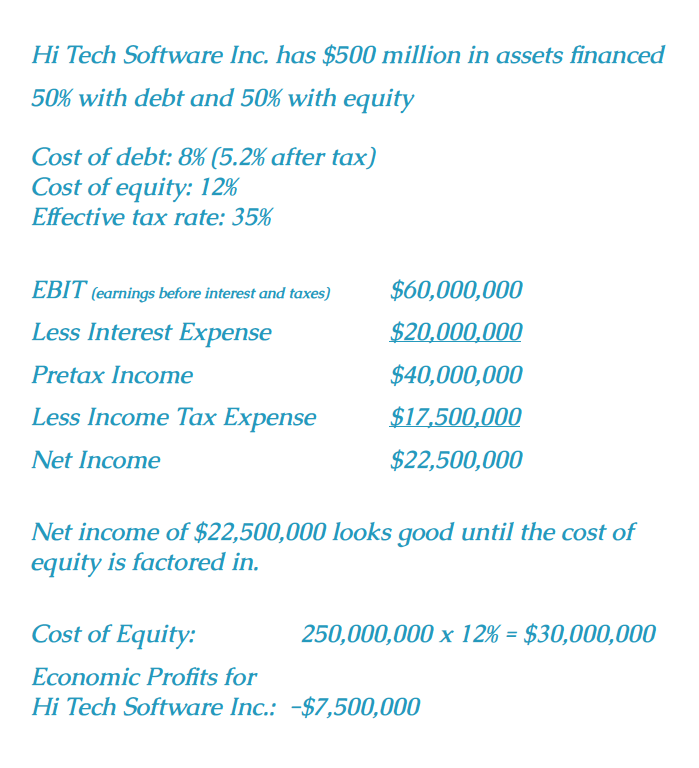
Hi Tech Software Inc. is profitable on an accounting basis, but unprofitable on an Economic Profits basis. The 12% cost of equity is an investor’s required rate of return, also known as the opportunity cost that a company must pay a shareholder to invest in the firm.
Why should investors subtract an amount for the cost of equity? Because if Hi Tech Software Inc. doesn’t deliver the investors’ required rate of return, they can choose another investment. In fact, investors can buy risk-free Treasury securities if the added risk of a given stock investment isn’t appropriately compensated by extra return. Although there is no legal requirement to deliver a return to equity holders (as there is for interest and principal paid to bondholders), firms must compensate for investment risk exposure in order to attract investors.
The Economic Profits Model has the additional benefit of slicing up cash flows to give us insight on whether management’s capital allocation decisions (dividend policy, share repurchase, acquisitions, etc.) create or destroy value over time. It is similar to modern corporate finance theory, whereby management teams strive to take on only projects that have a positive net present value.
A Real World Example
Let’s bridge the gap between the hypothetical and the real world by walking through a calculation of economic profits for technology giant, Oracle Corporation. The following example will take us through the steps of calculating economic profits. The equation for economic profits is as follows:
Economic Profit = Net Operating Profit after Taxes Minus Capital Charges
Step 1: Calculating Net Operating Profit After Taxes (NOPAT)
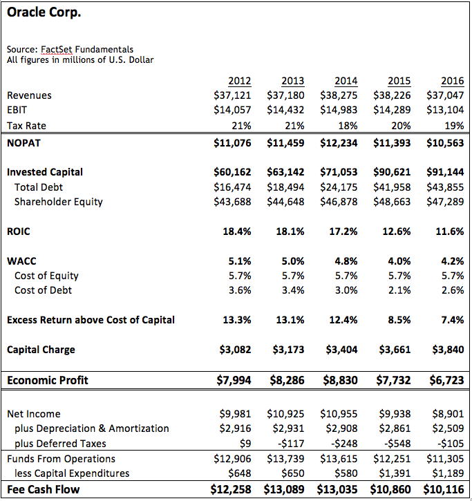
To calculate NOPAT, start with earnings before interest and taxes (EBIT) on the income statement and subtract the tax liability. Using the sample income statement in Figure 2 below, we calculated Oracle’s NOPAT for the fiscal years 2012, 2013, 2014, 2015 and 2016, as outlined in Figure 3 below.
Figure 2: Oracle Corporation Income Statement
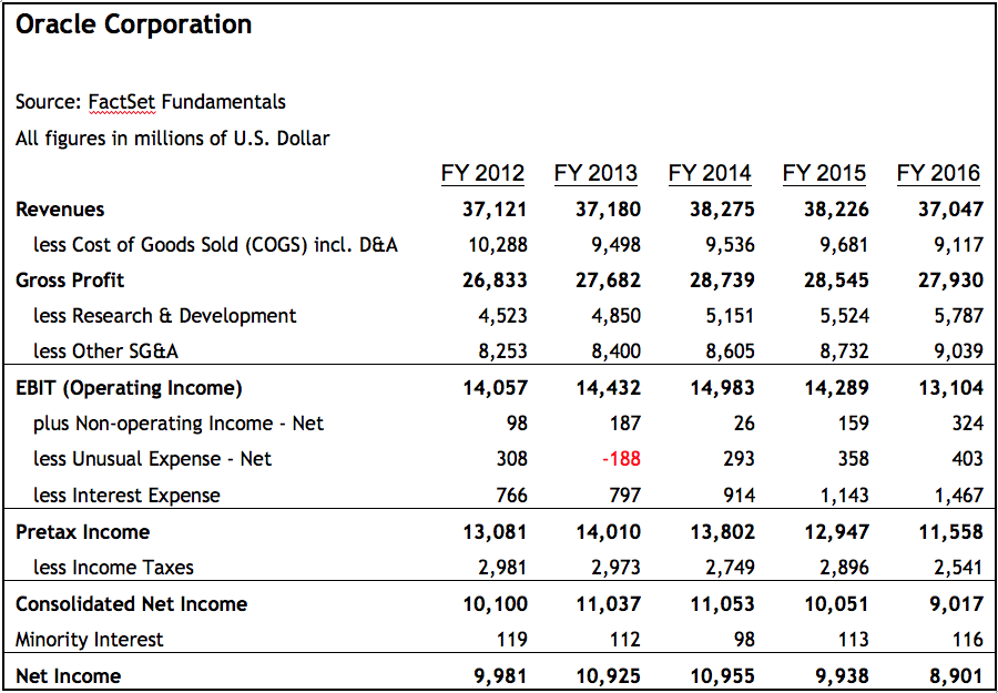
Source: Source: FactSet Fundamentals
Step 2: Calculating Invested Capital
After we determine NOPAT, the next step is to calculate the firm’s total invested capital – all money that has been invested in the company. This money provides the operating assets required for core business activities like inventory, property, plant, and equipment. There are a few different ways to calculate invested capital including the following:
Figure 3: NOPAT Calculation
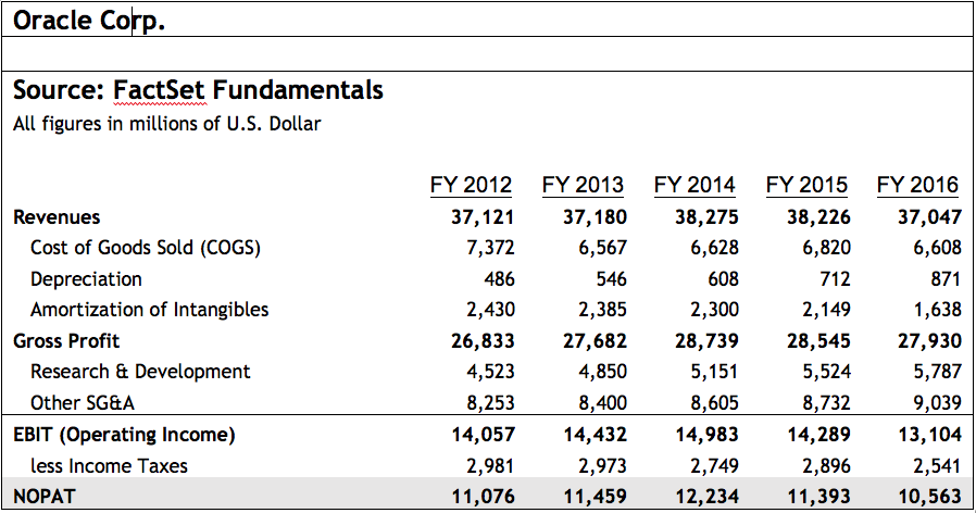
Source: Source: FactSet Fundamentals
Invested Capital
= Book Value of Debt + Book Value of Equity
= Fixed Assets + Current Assets – Current Liabilities – Cash
= Fixed Assets + Non-cash Working Capital
Invested capital is an estimate of the total funds held on behalf of shareholders, lenders, and any other financing sources. A key concept in the calculation of Economic Profits is that a company is charged “rent” for the use of these funds. Economic Profits then represents all profit in excess of this rental charge.
Continuing with the Oracle example, we calculate the firm’s invested capital at the end of 2016 as follows:
Invested Capital = Book Value of Debt + Shareholders’ Equity
= ($3.75 + $40.11) + $47.29 = $91.15
Step 3: Calculating the Cost of Debt
Because interest expense is deductible from income taxes, we define the cost of debt on an after-tax basis as follows:
Cost of Debt = (Interest Expense / Total Debt) * (1- tax rate)
= ($1.467 / ($3.75 + $40.11)) * (1 – 21%) = 2.6%
Figure 4: Oracle Corp. Balance Sheet
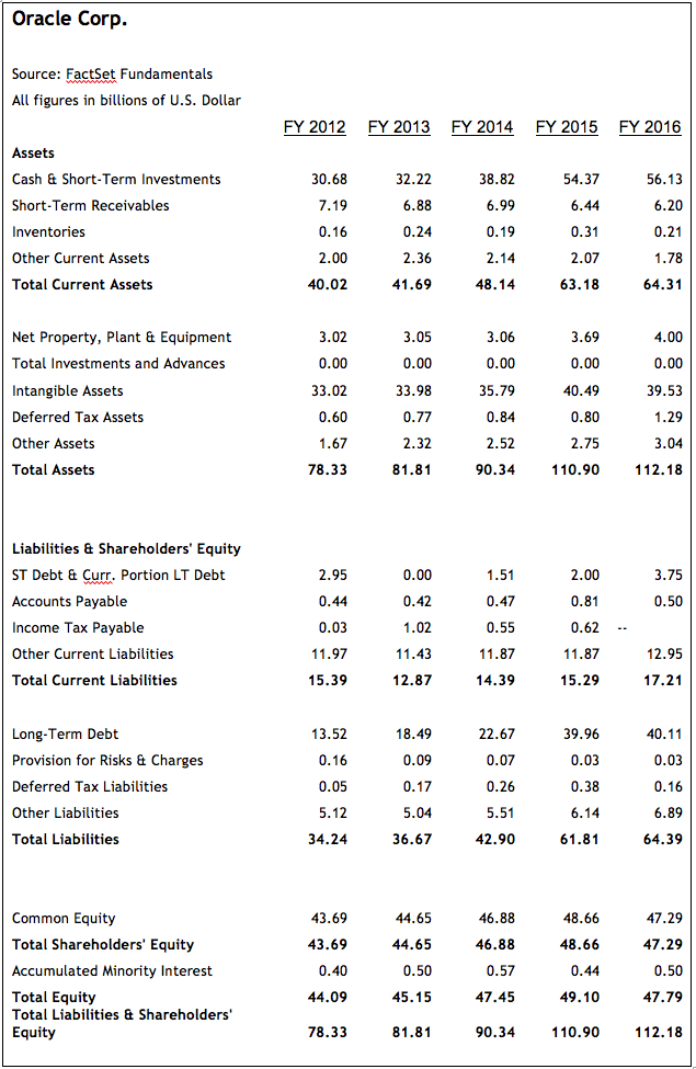
Source: Source: FactSet Fundamentals
Step 4: Calculating the Required Return on Equity
The required return on equity for an investment is the risk-free rate, such as a U.S. Treasury, plus a risk premium equivalent to the same risk as the investment under consideration. If a risk asset has an expected return equivalent to that of a risk-free asset, it would only make sense to buy the risk-free asset and avoid the risk asset.
When evaluating equities for potential investment we are interested in the rate of return an investor would require to hold the equity instead of the risk-free asset. This is referred to as the required return on equity and can be estimated using the Capital Asset Pricing
Model (CAPM).
Required Return on Equity= rf + β (rm – rf)
Where:
rf = the risk-free rate, typically the interest rate of the 10-year US Treasury
β = the trailing 3-year beta for the equity under consideration vs. the S&P 500
rm = the expected market return. A simple way to estimate this is by taking the expected earnings yield of the S&P 500, which is equivalent to the inverse of the price/earnings multiple of that same index
The (rm – rf) term is also known as the equity risk premium. This is the excess return an investor would require to hold equities instead of the risk-free asset. It has historically ranged between 3% and 5%.
Figure 5: Treasury Yields

Assume that we plan to hold an investment for the next 10 years. As of Feb 28, 2017, the forward 12-month P/E for the S&P 500 was 18.11x, which equates to an earnings yield of 5.52%. Another way to think about this is that investors expect the S&P 500 to return approximately 5.52% over the next 12 months. Using this information as well as the data from Figure 5, we can estimate the required rate of return for Oracle using the capital asset pricing model (CAPM) as follows:
Required Return on Equity= rf + β (ERP) = 2.50 + 1.07 (3.02) = 5.73%
Where:
Risk Free Rate (Rf) = 2.50%
Equity Risk Premium (ERP) = rm – rf = 5.52% – 2.5% = 3.02%
Beta (β) for Oracle (3-year trailing vs. S&P 500) = 1.07
Step 5: Calculating the Weighted Average Cost of Capital (WACC)
The weighted average cost of capital (WACC) is the rate of return that could have been earned by putting the same money into a different investment with equal risk. Thus, the WACC is the rate of return required to persuade an investor to make a given investment.
It is helpful to think of this as the investor’s opportunity cost of owning a particular investment. WACC is the rate that should be used to discount future cash flows to a present value. Companies that have well established business models, stable cash flows, manageable leverage, and a competitive edge should have a lower risk factor (β) than the market and thus a lower required rate of return.
Continuing with the Oracle example, we calculate the WACC as follows:
WACC = [(Debt/Total Capitalization)*Cost of Debt] + [(Equity/ Total Capitalization)*Cost of Equity]
= [($43.855 / $91.144) * 2.6%] + [($47.289 / $91.144) * 5.73%] = 4.22%
Step 6: Calculating Economic Profits
As we stated earlier, economic profits equal the firm’s net operating profit after taxes minus a capital charge. The capital charge is calculated by multiplying the total invested capital at the end of the period by the WACC as follows:
Capital Charge = WACC x Invested Capital
Capital Charge = 4.2% x $91,144 = $3,840
Figure 6: Calculating Economic Profits for Oracle Corp.
Source: Source: FactSet Fundamentals
Subtracting the capital charge from NOPAT we arrive at a value for economic profits:
Economic Profits = $10,563 – $3,840 = $6,723
Economic Profits for Oracle Corp. for the years 2012 through 2016 are summarized in Figure 6 below.
What can we take away from this example? In short, we see that Oracle created value for its shareholders over the five-year period. Not only did the company generate an impressive $59 billion in cumulative free cash flow, it also created in excess of $39 billion in Economic Profits, as a result of the positive spread between ROIC and WACC. Though this spread has narrowed (from 13.3% to 7.4%) over the last five years, it is still quite impressive. Positive economic profits indicate that management should continue to invest in the business as long as risk and return for future projects is similar to that of previous projects. If it continues to invest, Oracle should continue to generate positive economic profits and thus create wealth for its shareholders.
On the other hand, if economic profits were negative, Oracle management should consider shifting investment from projects with negative economic profits into those with positive economic profits or, if no such projects are identified, the company should return capital to shareholders through stock buybacks or dividend payments. Oracle may also consider acquiring a company or division with higher economic profits than it produces internally, but only if it pays a reasonable price for those assets. The bottom line is – only take actions that result in positive economic profits. If a management action results in negative economic profits, it will ultimately destroy value for shareholders, and the company’s price will decrease.
Let’s consider another example, Valeant Pharmaceuticals (VRX). Using the same methodology as the previous Oracle example, we have calculated the company’s free cash flow and Economic Profits in Figure 6 below. At first glance, it appears that Valeant has created over $4 billion in value for shareholders over the five-year period, based on free cash flow. However, using the Economic Profits Model, we see that Valeant actually destroyed wealth for shareholders in all but one year. In total, the company destroyed over $2.8 billion in shareholder wealth. This example highlights the importance of considering capital structure when choosing investments. Recall that DCF models only subtract the cost of debt by deducting interest expense from operating income. Economic Profits also factor the cost of equity into the equation.
The examples of Oracle Corp. and Valeant Pharmaceuticals show how useful the Economic Profits Model can be in assessing whether management’s prior capital allocation decisions have created or destroyed wealth for shareholders. However, the Economic Profits Model is also useful as a valuation tool to assist in determining a company’s intrinsic value, which can then be used to derive a fair value for the firm’s equity. The Economic Profits Model is the primary valuation tool we employ at QSV Equity Investors.
Economic Profits as a Valuation Tool
Economic Profit is based on the same idea as discounted free cash flow. However, with the Economic Profits Model, the firm’s total value is broken into two parts: invested capital and the present value of future economic profits. The sum of these two parts equals the firm’s intrinsic value. The theory behind economic profits was developed by Bennett Stewart in the 1980s and presented in his best-selling book, The Quest for Value.
Figure 7: Economic Profits for Valeant Pharmaceuticals
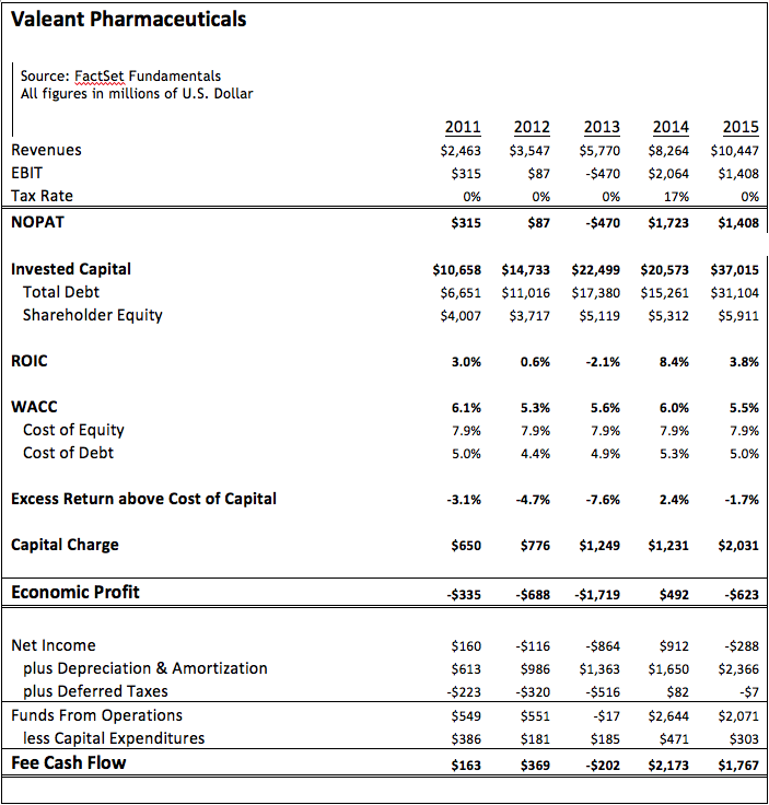
Source: Source: FactSet Fundamentals
Figure 8: Using Economic Profits as a Valuation Tool
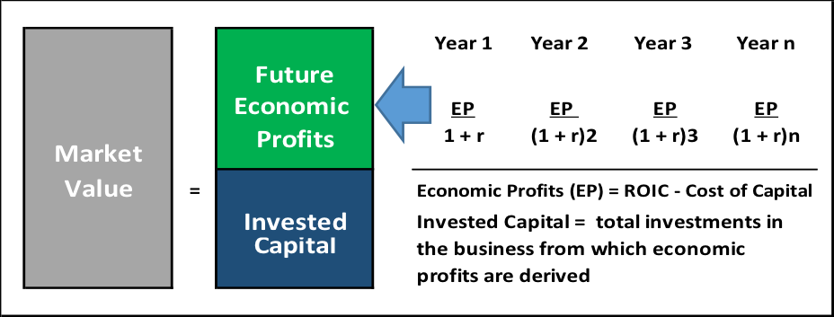
The Value of a Firm = Invested Capital + Present Value of Future Economic Profits
Economic profit is profit after all costs, including the cost of borrowing investors’ funds. If economic profit is increasing, then the firm’s intrinsic value is also increasing, suggesting that market value should
also increase.
Recall that the Economic Profits and Cash Flow Models arrive at the same intrinsic value for a company. However, we believe the Economic Profits Model provides additional insight into whether management’s capital allocation decisions are creating or destroying value, which makes this model a better choice for valuing a firm.
Of course, the limitation on both models is that they are only as good as the data input into the model. In other words, garbage in/garbage out. Both models require successfully forecasting a number of variables in order to arrive at an accurate firm value. Admittedly, this can be more art than science. However, we believe that in the hands of experienced investment professionals the Economic Profits Model can be a powerful tool in determining a company’s intrinsic value.
Let’s continue with our earlier Oracle analysis. This example oversimplifies the process, but still provides a reasonable overview of the methodology. For this example, we have made the following assumptions:
- Revenues are projected to grow at 3% for the first five years and then drop to 2% thereafter.
- EBIT margins start at 35%, consistent with fiscal year 2016, and subsequently decay by 1% per year.
- Tax rate is assumed to be in line with the 10-year average at 25%.
- Total debt is assumed to remain constant.
- For simplicity, WACC is assumed to remain constant at 6%. In reality, this number changes over time as the capital structure changes and interest rates fluctuate.
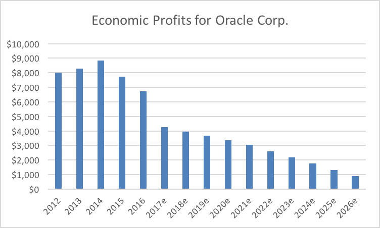
Using the set of assumptions above, we can project Oracle’s economic profits well into the future as shown in Figure 9.
It’s important to note that economic profits peaked in 2014 and, based on the data presented here, are projected to trend down until 2026. This means that Oracle is expected to generate ROIC greater than its cost of capital until 2026 and after that point level off.
Calculating Terminal Value
When building a valuation model, there is a stated forecast period for which analysts make very detailed assumptions about a firm’s future growth and profitability. As investors, we would all like to own companies that grow economic profits at an attractive rate forever, well beyond our forecast period. However, the reality is that most if not all firms eventually settle into a steady state where the spread between ROIC and WACC stabilizes. This does not mean the firm no longer grows, it simply signifies a transition into middle age and maturity. An effective valuation model must account for this transition period.
To account for this transition period beyond the stated forecast period, we rely on concept known as Terminal or Continuing Value. Terminal Value represents future economic profits far into the future, discounted back to the present.
Terminal Value = ((ROIC – WACC) / WACC) / (1+WACC)n
If we determine that economic profits are positive during the transition period, the terminal value will be positive and add to the intrinsic value of the firm. If economic profits are zero, meaning ROIC = WACC, the terminal value will equal zero and will have no effect on intrinsic value. Lastly, if ROIC is less than WACC, the firm is expected to destroy value and will decrease the current intrinsic value of the firm.
The length of a model’s stated forecast period determines what portion of a firm’s total value is attributable to the Terminal Value. The shorter the stated forecast period, the greater the percentage of total firm value attributable to Terminal Value, and vice versa. Typical forecast periods range from 5 to 20 years. At QSV, we prefer to use a 20-year period. Although it can be more challenging to accurately forecast that far into the future, a 20-year period allows us to adequately factor mean reversion into our models and to taper the ROIC toward the cost of capital over time. A longer period also allows us to vary the competitive advantage period and evaluate multiple growth scenarios. To simplify the Oracle Corp. example, we shortened the stated forecast period to 10 years. Beyond that forecast period, Oracle still generates profits. Terminal Value is how we estimate what these future undetermined profits are worth.
The most commonly used method of establishing a Terminal or Continuing Value is to assume that the Economic Profits generated in the final year of
Figure 9: Economic Profit Valuation for Oracle Corp.
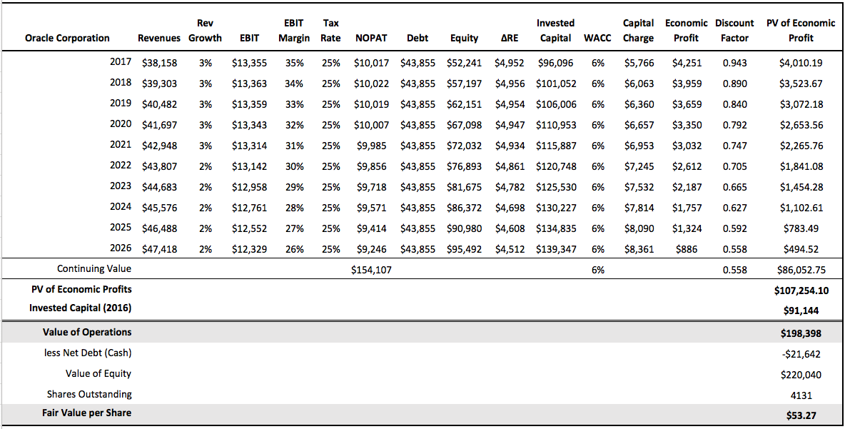
Figure 10: Economic Profits
the stated forecast period remain constant going forward. Those Economic Profits are then divided by the final year WACC to arrive at a Terminal Value for the company. This is a very conservative method of estimating Terminal Value, and in many cases, understates a company’s value. However, because we are using a 20-year forecast period and because we build a significant amount of mean reversion into our models, we are comfortable that our approach reasonably reflects the middle-age or mature years that lie ahead for the company. To continue with the Oracle example, we calculate a terminal value of $154,107 ($9,246/6%) for the company.
The Final Step: Intrinsic Value
At this point in our stock evaluation process, we have calculated a series of values for an individual company: future Economic Profits for the stated forecast period and a Terminal Value for the company beyond that period. In order to use this information to determine the company’s current value, we take the present value of each of these cash flows by discounting at the WACC as shown above in Figure 9. Adding together the discounted values of each stream of cash flows gives us the present value of future Economic Profits.
In the Oracle example above, the present value of Economic Profits equals $107,254 ($21,202 + $86,052).
There is one final step in determining a company’s intrinsic value. Recall that a company’s fair value is equal to the sum of its total invested capital plus the present value of future economic profits. Returning to the Oracle example, we must therefore add the current year invested capital ($91,144) to the present value of future Economic Profits ($107,254).
This yields an intrinsic value of $198,398 billion for Oracle Corp., which is the dollar amount a potential buyer should be willing to pay for the entire company.
Total Invested Capital + PV of Future Economic Profits = Intrinsic
or Fair Value
$91,144 + $107,254 = $198,398 billion
As equity investors, we want to know how this translates to a fair value for an individual share. Therefore, we subtract the net debt and divide that value by the number of outstanding shares. In the case of Oracle, we would estimate the fair value to be around $53 per share as follows:
Fair Price per Share = (Intrinsic Value – Net Debt) / Shares
Outstanding
= ($198,398 – (-$21,642)) / 4131 = $53
Since the stock’s intrinsic value is $53, investors should consider buying the stock when it trades for less than $53 and selling or shorting it when it trades above $53.
Conclusion
Based on years of investing experience and our understanding of common investor behaviors, we believe there are two primary hurdles that prevent people from being successful investors. The first is the inability to separate day-to-day stock price gyrations from underlying company fundamentals and the second is the tendency to buy stocks when they are priced above value, have returns that are reverting to the mean, and carry higher risk than expected. Conversely, thinking like business owners rather than a stock investors and owning stocks when they are trading below their intrinsic value are two notable advantages for investors.
At QSV, we purposefully act like business owners, focusing on a company’s intrinsic value and blocking out day-to-day price moves. Our stock selection process uses a variety of valuation measures to screen for potential investment opportunities. We then rely on an Economic Profits Model to determine whether a company is able to create wealth, what the company will be worth well into the future and what is a fair price for the company in the present. That is how we decide whether or not we want to own a stock. We believe the Economic Profits Model is a powerful tool for choosing stocks that will help our clients beat inflation and create long-term wealth.
Bibliography Stewart, G. Bennett. The quest for value. Harper Collins, 1991.

Competitive Advantage Period Defending Your Castle
QSV_Competitive Advantage Period
“In business, I look for economic castles protected by unbreachable ‘moats’. The wider a business’ moat, the more likely it is to stand the test of time.” -Warren Buffett
Companies that generate returns on invested capital greater than its cost of capital are instrumental in achieving long-term wealth for investors, as discussed in our previous paper, “A Valuation Framework for Beating Inflation and Creating Long-Term Wealth.” Unfortunately, companies that create wealth eventual
ly attract competition from other companies, ultimately driving down product prices and profit margins.
Competition and lower prices are good for consumers and society as a whole, but can be detrimental for individual companies’ profitability. Many investors fail to appreciate this reality and are surprised when the stock of a previously successful company reverts downward.
This scenario is common with small-cap growth companies. Typically, a small company with an exciting new product (such as a smartphone app) grows very rapidly in the beginning, ultimately driving up its stock price and valuation. Other companies, having observed this successful product, copy the idea, quickly encroaching into the same space. This usually leads to an unfavorable earnings surprise for the original innovator and the stock gets crushed when the market figures out what has happened. Compounding the impact is that these stocks are typically long duration stocks, which means investors place more value on cash flows in the distant future and less value on current cash flows and earnings. Such stocks are commonly referred to as “story” stocks, but sadly many stories never materialize because competition is alive and well in the world. Imagine that — capitalism works.
Because competition is real, it is important for investors to assess the competitiveness of every company in their portfolio. On the positive side, many companies have the ability to generate positive economic profits for many years before eventually reverting back to the cost of capital. Most likely, these companies have created competitive advantages that prevent other companies from eroding all of their excess returns.
Warren Buffet calls such competitive advantages “economic moats” and consistently emphasizes that he wants to own businesses that are like a castle surrounded by a moat that can fend off competition. Historically, moats were deep, broad ditches, typically filled with water and surrounding a castle, building or town. Moats provided a preliminary line of defense against enemies and invading armies. An economic moat is like a castle moat, but instead of fending off Romans or Huns, a company’s “moat” helps it fend off competing companies. Any advantage a company has that acts as a barrier preventing other companies from stealing market share and profits is referred to as its competitive advantage.
Competitive Advantage Period (CAP)
Companies with a positive economic spread, meaning the companies earn a return on invested capital in excess of capital costs, will eventually attract competition. This is where investors’ real work begins. Once we identify companies with high returns on capital, we need to determine whether those companies have competitive advantages and how durable those advantages are.
Determining how durable and how protracted a company’s Competitive Advantage Period (CAP) will be is key to successful valuation. We want a CAP that lasts far more than a year or two. Ideally, we want CAPs that last 10, 15 or even 20 years. Stocks with long CAPs that are bought at reasonable valuations can produce attractive returns and great wealth for investors well into the future. Companies with long CAPs should trade at higher multiples than their peers. However, many companies with short CAPs trade at high multiples due to the market’s infatuation with earnings growth and story stocks.
“In spite of CAP’s importance in the analytical process—it remains one of the most neglected components of valuation.” – (Mauboussin, et al., 1997).
Companies with long CAPs can be held for many years, thereby reducing trading costs, capital gains taxes, and market timing mistakes. High CAP stocks are justly labeled “sleep at night” stocks. For example, suppose a company like Coca-Cola misses an earnings estimate. Immediately, analysts publish negative reports, causing investors to panic and sell the stock. But investors who did their homework know that Coke has a very long competitive advantage period due to its tremendous brand identity and scale. These investors are likely to recognize the stock’s decline as a buying opportunity. In contrast, if a speculative technology company misses its earnings, investors would need to quickly determine whether new entrants had broken through and permanently reduced the company’s future prospects and profitability. A strong business does not survive from quarter to quarter, and one bad earnings announcement should not change the long-term outlook of a quality company with high future economic profits.
The concept of CAP is not new. In fact, it dates back to 1961, when Modigliani & Miller wrote their paper, “Dividend Policy, Growth, and the Valuation of Shares.” In this paper, they asserted that a company’s special investment opportunities would not last in perpetuity, but over some finite interval. They defined CAP as follows:
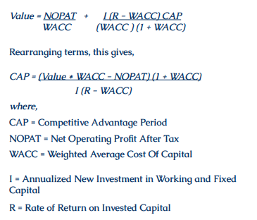
In his 1997 paper, “CAP – The Neglected Value Driver,” Michael Mauboussin points out that as time goes on, competitive forces drive returns to a level approaching the cost of capital. He graphically illustrates CAP in three figures very similar to Figures 1, 2 and 3 below, where the vertical axis is the percentage of economic profits (return on invested capital less the cost of capital) and the horizontal axis is time. The shaded area under the curve represents the incremental value that management has created for shareholders. As we explain in our paper, “A Valuation Framework for Beating Inflation and Creating Long- Term Wealth,” this is what the market should focus on in order to determine whether or not management creates or destroys value over time.
When creating a discounted Economic Profits Model, investors should estimate how long the CAP will last. To effectively do this, one must assess the competitive dynamics of the industries in which the company competes. The most commonly used framework, and we believe the gold standard for this analysis, is Michael Porter’s five competitive forces. Porter was a pioneer in the development of competitive strategy in his revolutionary 1980 book “Competitive Strategy: Techniques for Analyzing Industries and Competitors.” (Porter, 1980). We intend to dive deeper into the topic of competitive dynamics in our next paper. In the meantime, Porter’s five forces can be summarized as follows:
- Threat of new entrants – the higher the barriers to entry, the longer the CAP and vice versa
- Threat of substitutes – the lower the threat of substitutes, the longer the CAP
- Bargaining power of customers – the lower the customers’ bargaining power, the longer the CAP
- Bargaining power of suppliers – the lower the suppliers’ bargaining power, the longer the CAP
- Industry rivalry – the lower the industry rivalry, the longer the CAP
Short Competitive Advantage Period
A Short Competitive Advantage Period (in Figure 1 five years) would be typical for industries that exhibit traits of perfect competition. Perfect competition is a theoretical market structure used as a benchmark against which real-life market structures are compared. In real life, the industry that most closely resembles perfect competition – and would, therefore, exhibit short to no CAP – is agriculture. A farmer goes to market with corn or wheat and takes whatever price the commodity sells for on the exchange. Because the farmer’s crop is identical to all others, the farmer cannot affect the price. No one farmer has a large market share, and no matter how much a farmer sells into the market, it will not change the price. In such a market, it would be difficult if not impossible for any individual farmer to gain any type of competitive advantage versus other farmers. Under perfect competition, there are many buyers and sellers, and prices reflect supply and demand. Consumers have many substitutes if the product or service they wish to buy becomes too expensive or quality falls short. For example, if beef is too expensive, consumers can switch to chicken or pork. Furthermore, new firms can easily enter the market, increasing competition. If corn is more profitable than soybeans, a farmer can switch between plants each year. Companies earn just enough profit to stay in business and no more. If farmers were able to earn excess profits, other companies would enter the market or switch crops and drive profits back down to the bare minimum. If prices remain too low for a period of time, farmers would get out of the market or switch to more profitable crops. Companies that sell commodity type products with no specific attributes will earn no economic profits and operate at or near the industry cost of capital. Thus, their competitive advantage period is virtually non-existent.
Figure 1 – Short Competitive Advantage Period
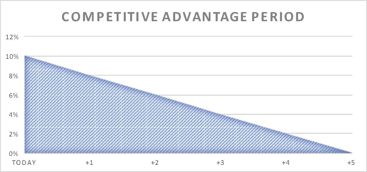
Source: QSV Equity
Other industries operate with very short CAPs. An example is electronics manufacturing services (EMS). The EMS industry resides at the bottom of the technology supply chain due to low technology differentiation, aggressive bidding for new business programs, and inferior margins. Barriers to entry in EMS are very low, allowing countless competitors across the globe to compete for business. Customers, therefore, hold considerable negotiating leverage and continually demand more services and/or lower prices to retain their business. As a result, EMS firms, such as Sanmina, Flextronics and Jabil, compete largely on price, which limits their ability to improve profitability and earn their cost of capital.
The EMS industry faces a vicious environment where firms are continually required to provide more services for less money. Such unfavorable dynamics keep a ceiling on the profitability potential of competitors within this industry. As a result, many EMS companies find it increasingly difficult to generate returns above their cost of capital. Competitive advantages are very difficult to obtain in the EMS industry, which means that even a five-year CAP might be generous.
Long Competitive Advantage Period
At the opposite end of the CAP spectrum is a monopoly, where a single company or group owns all or nearly all of the market for a given type of product or service. By definition, monopoly is characterized by an absence of competition, often resulting in high prices and possibly inferior products due to lack of incentive for innovation. There are very few true monopolies in real life. Utilities are considered monopolies if there is only one provider
in a certain area, but even here, government typically regulates what the utility is able to charge. Such
monopolies may enjoy very long competitive advantage periods, but would still achieve slim excess returns above the cost of capital. For individual companies, the best strategy is to position themselves in a profitable industry with some type of advantage to stifle competition.
Figure 2 shows how the CAP may last well into the future if a company possesses a competitive advantage that makes it hard for competitors to copy. The value creation period (shaded area) is much longer for this type of company.
An example of an industry with a long CAP is the system software industry, which exhibits significant competitive advantages due to high switching costs. Companies possess this advantage if buyers face significant inconvenience or expense to change
Figure 2 – Long Competitive Advantage Period
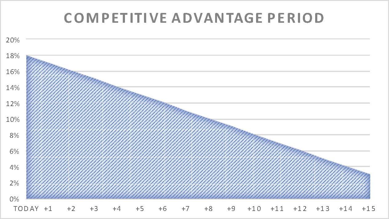
Source: QSV Equity
from their products to another provider. In such cases, a competitor would have to offer substantial improvement in price or performance to motivate users to make a change. Consider how difficult it would be to switch your Microsoft Windows to a competitor’s operating system. It most likely isn’t worth the hassle for any potential savings or expanded capability.
High switching costs are an example of a barrier than can act as a moat, protecting a company from competition. These one-time costs for a buyer switching from one supplier’s product to another’s may include employee training costs, the price of new equipment, time invested in testing or qualifying a new product, need for technical expertise, product redesign, and lost production during a transition from one product to another. The higher these costs, the less prospect of a customer switching to another supplier. This is why customers tend to stick with their current technology and grudgingly pay yearly increases in maintenance or subscriber fees.
Typical Competitive Advantage Period
In the real world, the CAP period may not be as uniform as the theoretical presentations in Figures 1 and 2. Rather, Figure 3 may be a more realistic representation. A company may have negative economic profits in the early stages as it invests heavily in new projects. Economic profits then eventually turn positive for a number of years as returns on those projects pay off. Then eventually economic profits revert back toward the cost of capital as the company matures or other competitors enter the industry. This is similar to a typical business cycle
Conclusion
In practice, it can be difficult to pinpoint a specific numerical value for CAP. Nonetheless, qualitatively, CAP is extremely useful in the development of financial models. Attention to CAP forces analysts to carefully consider where a company and its industry are in the business life cycle. Awareness of CAP also places greater focus on the competitive landscape. We know that for the vast majority of companies, return on invested capital tends to converge toward their cost of capital over time. Carefully assessing an industry’s competitive landscape and weighing the sustainability of a company’s CAP can greatly improve the efficacy of a valuation model, thereby improving long-term portfolio returns.
Figure 3 – Common Competitive Advantage Period
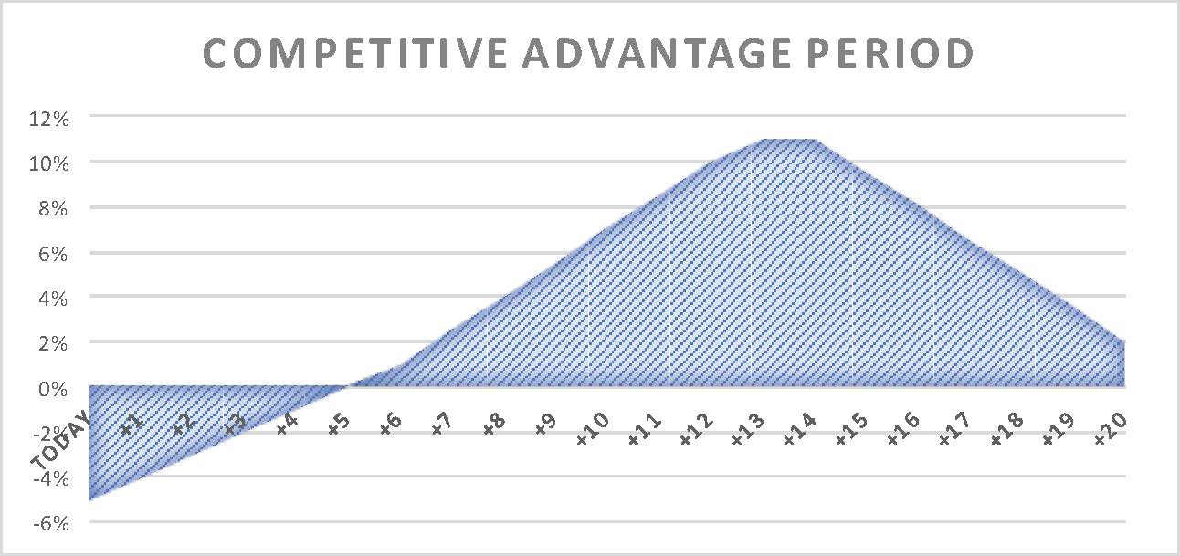
Source: QSV Equity
Bibliography
Porter, Michael E. Competitive strategy: Techniques for analyzing industries and competitors. Simon and Schuster, 2008.
Miller, Merton H., and Franco Modigliani. “Dividend policy, growth, and the valuation of shares.” the Journal of Business 34, no. 4 (1961): 411-433.
Mauboussin, Michael, and Paul Johnson. “Competitive advantage period: the neglected value driver.” Financial Management (1997): 67-74.

The Myth of High Beta
“Can investors forego short-term thrill for long-term reward?”
In a rational investment market, investors demand higher returns to compensate for higher risk. Therefore, one should logically expect lower returns from safer securities and higher returns from riskier securities. This has long been one of investing’s fundamental precepts. However, rational is not always an accurate description of investor behavior. This paper questions the long-held belief – some would say myth – that higher risk, high beta stocks deliver the highest returns. Furthermore, we present studies that show how the “low volatility anomaly” creates opportunities to beat the market and create long-term wealth.
Market Efficiency and the Value of Active Management
In order for people to believe they (or their professional money manager) can beat the market, they must start with the notion that markets are mostly, but not always efficient. If the stock market were perfectly efficient, it would be futile to pay an active money manager. A low-cost index fund would certainly be the best alternative.
Though the aggregated performance of professional investment managers may at times support a case for index funds, a deeper understanding of market dynamics and investor psychology reinforces the potential value of active management and may help investors determine which managers and strategies are better suited to beat the market.
For active managers to gain an edge, there must be market anomalies or inefficiencies. These anomalies must not only exist in the short term but also persist over the long term. In our view, some of the same human behavioral biases that cause investor error also allow anomalies to recur time and time again. In this paper, we discuss investors’ love affair with high beta stocks, as well as the low beta/low volatility anomaly and the natural human tendencies that sustain it. Most importantly, we show how this anomaly creates opportunities to outperform the market with less risk, casting doubt on the well-entrenched myth that high beta stocks are the surest path to higher returns.
The Efficient Market Hypothesis Requires Rational Investor Behavior
Known for his Journal of Finance article, “Efficient Capital Markets: A Review of Theory and Empirical Work,” Nobel Prize Laureate Eugene Fama theorizes that all information is already reflected in all stock prices, thus making it impossible to outperform the market (Fama, 1970). According to the Efficient-Market Hypothesis (EMH), stocks always reflect all available information, eliminating any possibility of purchasing undervalued stocks or selling stocks at inflated prices. If the hypothesis holds, investors – whether professional or not – should be unable to outperform the overall market through stock selection or market timing. The only way investors could obtain higher returns is by taking on additional risk through high beta stocks.
There are many models that attempt to explain the risk-reward relationship of stocks relative to the market portfolio. The Capital Asset Pricing Model (CAPM), which uses a single factor (beta) to explain pricing and asset returns, was a remarkable breakthrough in finance that won William Sharpe the 1990 Nobel Prize in Economics. Unfortunately, beta alone has not done a very good job of explaining observed market risk and returns.
In order for the EMH to hold, investors must be risk-averse and always make rational investment choices. This assumption doesn’t always prove true, however, and many academics have tried to explain why. This has spawned an area of study known as behavioral finance or behavioral economics. Behavioral finance grew from the idea that individuals aren’t always rational and quite often make irrational decisions. There have been many studies on behavioral finance by psychologists such as Daniel Kahneman, Amos Tversky, and Richard Thaler to name just a few. Behavioral economists attribute imperfections in financial markets to a combination of cognitive biases, some of which we’ll review in this paper.
Stock Market Bubbles: Collective Wisdom or Irrational Decision Making?
Stock market bubbles are a notable outcome of irrational decision making. Bubbles occur when market participants drive stock prices above their value relative to some system of stock valuation. In the 20th century, the stock market experienced a number of bubbles, including the bubble that preceded the Great Depression and the dot-com Bubble of the late 1990s. Both were fueled by speculative activity involving new technologies. The 1920s saw amazing innovations including radio, automobiles, and aviation. In the 1990s, the Internet and e-commerce technologies emerged.
Some analysts, affirming crowd-sourced wisdom, theorize that price movements, even bubbles, really do reflect rational expectations of fundamental returns. Behavioral finance theory, on the other hand, attributes stock market bubbles to cognitive biases, including the tendency to overpay for excitement, herd instinct, regret avoidance and other common human tendencies. There’s also a more cynical school of thought that one can make money buying securities, whether overvalued or not, because there will always be someone (a greater fool) who is willing to buy that stock at a higher price. In our view, stock market bubbles provide clear evidence that investors do not always act rationally.
Investors’ High Beta Addiction
Whether we like to admit it or not, we all probably agree that the latest, greatest smartphone or a new social media company is much more exciting (though not necessarily more profitable) than a company that sells salad dressing or creates software for government agencies. In general, financial news is not the most exciting subject matter, so it’s no surprise that financial newscasters spice up their reports and juice their ratings with news of exciting high growth companies. Investors too are beguiled by what are typically classified as “high beta” stocks and sometimes referred to colloquially as “glamor” or “speculative” stocks.
Stocks are tagged as high beta when they exhibit high growth and high price momentum. These stocks are expected to rise more than the overall market in good times and fall more than the market in bad times. They may involve specific speculative risks, for example, uncertainty about an event that may produce either a profit or loss. However, investors who own these stocks are all too willing to take on added risk in hopes of a commensurate payoff. Let’s look at some of the behavioral biases behind this attraction.
Blackjack, Baseball and Beta – Why People Overpay for Excitement
Looking at irrational gambling behaviors may shed some light on why investors prefer high beta stocks. Think about someone who gambles online or loses significant sums playing blackjack at a casino. They very likely view gambling as a low-risk, high-yield proposition. In reality, it’s the opposite: a high-risk, low-yield proposition. The payouts of every casino game always favor the casino which is called the “house edge” or “house advantage.” For example, for each bet on the roulette wheel, the casino keeps 5.26% of winnings on average. Blackjack, the most popular table game, returns a bit more in winnings than roulette, but it too is subject to what is called the house edge. Yet, according to The Wall Street Journal, the U.S. still spent $104.1 billion on gambling in 2015 (WSJ 2016). The thrill of hitting a casino jackpot is often just too alluring – despite its improbability. Excitement and anticipation create a natural high, an adrenaline rush. Studies show that people get this same feeling when buying exciting high momentum growth stocks.
Three experts in the field of Neuroeconomics, Wolfram Schultz, Read Montague, and Peter Dayan have written studies showing that financial gains trigger the release of dopamine, a brain chemical that stimulates a natural high. The studies have shown that the less likely or predictable a financial gain, the more dopamine is released and the longer it affects the brain. This may explain why gamblers are drawn to low-probability bets with high potential payoffs. When such bets pay off, they produce an actual physiological change; a massive dopamine release floods the brain with a soft euphoria. Through the use of MRI technology, Schultz and Montague also found similarity between the brains of people who have successfully predicted financial gains and the brains of people addicted to morphine or cocaine. After a few successful predictions, financial speculators can literally become addicted to the dopamine release.
A person with high dopamine levels typically becomes over-confident and tends to take undue risk. This may cause gamblers to wrongly attribute success to their own prowess or “system” rather than luck. Addiction to the dopamine kick may keep them playing until they lose all their money. Similarly, some investors become “addicted” to hot high beta speculative stocks. The excitement triggers dopamine. On the other hand, successful investors like Warren Buffet often make money in boring industries like insurance, finance, railroads, food, and beverage. With less excitement, there’s likely less risk of dopamine over-riding one’s more rational decision-making abilities.
Turning to baseball, another popular U.S. pastime, the bestselling book “Moneyball: The Art of Winning an Unfair Game” by Michael Lewis provides a concrete example of overpaying for excitement. While most Major League Baseball teams hired expensive home run hitters that fans loved to watch, Oakland Athletics general manager Billy Beane favored an analytical, evidence-based approach to assembling a competitive team. Oakland hired undervalued players who more consistently got on base with a walk or a single. Even though sabermetrics (the empirical analysis of baseball stats) clearly indicated that on-base percentage was critical to offensive productivity, the baseball labor market seriously undervalued that factor.
Overpaying for home runs and underpaying for walks and singles is quite similar to investors’ preference for “speculative/ high beta” stocks over stocks that deliver singles year after year. Many believe the Moneyball anomaly corrected once it was exposed, which may be true since there are only 30 MLB teams. However, in order to correct a parallel anomaly in the stock market, millions of “players” would have to be persuaded to forego the thrill of buying speculative high beta stocks.
There are a number of other human tendencies that may contribute to investors’ preference for high beta stocks. These include:
- The Lottery Effect: Like casino games, lotteries are high risk, low yield games. According to the Multi-State Lottery Association, which oversees the Powerball Lottery, the odds of matching all numbers is 292,201,338 to 1. Payouts from lotteries are even worse than casinos, as states take a cut of total receipts to support government expenditures. In Illinois, for example, lottery receipts totaled $2.84 billion for Fiscal Year 2015. Of this amount, only 64% of gross lottery revenue is actually paid out in prizes. The rest goes to expenses associated with running the lottery and state capital projects. Why then is the lottery so attractive to so many people? One reason is that people tend to (optimistically) assign more weight to the probability of winning than is justified objectively. Second, people like the idea of spending a very small amount with the possibility (no matter how slight) of winning big. Similarly, many investors are attracted to low-priced, high-risk stocks for the slight possibility of jackpot size returns.
- Herd Instinct: Nobody wants to miss a great opportunity and when a stock is rising, everyone wants to be on the bandwagon. Being a contrarian or value investor isn’t as easy or fun as buying trendy stocks. It’s hard work determining why a stock is out-of-favor, whether it has reached its lowest price, when or if the company will fix its problems and if that company has sufficient liquidity to survive in the interim. Even when investors believe a company’s problems are temporary, it’s psychologically difficult to watch a stock make new lows or to continually add to a stock that keeps missing earnings. It’s much easier to join in the pep rally for a stock on its way up. This is true even for professional investors, who find safety in numbers. In practical terms, a manager is less likely to be fired when other investors and fund managers are buying the same favored stocks.
- Regret Avoidance: What were people thinking in 1999 when stock prices entered astronomical territory? Many clearly believed stocks would keep rising and didn’t want to miss any of the ride. People often stick with a high flying stock to avoid the regret of selling too soon. How would they feel if they had sold in 1997 only to see the market go up for two more years?
- Faulty Extrapolation: A tendency to extrapolate the current situation – whether good or bad – leads investors to over penalize companies with short-term issues, erroneously believing the bad news will have a larger and longer impact than it actually does. Similarly, investors too often extrapolate recent good earnings growth too far into the future. This leads to under-discounting stocks with current earnings momentum.
- The “Hot Hand” Effect: Like blackjack players with a “hot hand,” investors may attribute too much of their success to their own abilities. Furthermore, the good feeling associated with winning may fuel unfounded optimism that success will continue. Unfortunately, this may persuade investors to commit even more money to the market, all too often at cycle peaks when stocks are most expensive.
The Low Beta/Low Volatility Anomaly
So far we have focused on why investors are so attracted to high beta stocks. Let’s now consider whether they are rewarded for their devotion. The notion that high beta stocks should earn higher average returns than low beta stocks has been a cornerstone of modern finance. In an efficient market, investors should enjoy above-average returns only when they take above-average risks. In reality, this isn’t always the case. Over the last 20 years, there has been a significant academic investigation into the relationship between volatility and performance. Study after study has concluded that investors are not appropriately rewarded for taking either systematic (beta) or idiosyncratic (company specific) risk.
There is a persistent anomaly in the risk/return trade-off between high and low beta stocks. Portfolios of low-volatility stocks have produced higher risk-adjusted returns than portfolios of high-volatility stocks. For investors, this is a sort of “Holy Grail” – higher returns with less risk.
The outperformance of low beta stocks and portfolios is not a new discovery. In addition to academic evidence, which we review below, there’s also a growing interest on the part of investors. Following the dot.com bust and the financial crisis of 2008, baby boomers have been burned in the market too many times and seem to be more emotionally ready to tone down the “excitement” in their portfolios in the interest of preserving their hard earned money for retirement.
Academic Support for the Low Beta Anomaly
As early as 1972, Jensen, Black, and Scholes demonstrated that the expected excess return on a security was not linearly related to its beta (Jensen, et al., 1972). The authors found that high beta stocks have negative alphas (i.e. are overvalued) and low beta stocks have positive alphas (are underpriced). Fama and French also observed a weak positive relationship between average return and beta. Low-beta portfolios had average returns that were similar or higher than those of high-beta portfolios (Fama, et al., 1992).
- “Benchmarks as Limits to Arbitrage: Understanding the Low-Volatility Anomaly” One of the better studies on this subject comes from Baker, Bradley, and Wurgler (Baker, et al., 2011). Their study points to low beta as one of the greatest anomalies in finance. The authors find that “over the 1968 to 2008 period, low-volatility and low-beta portfolios offered an enviable combination of high average returns and small drawdowns [less risk].” Figure 1 shows the return of $1 invested in 1968 in each of five quintiles of stocks divided by volatility and beta measurements. The bottom quintile (or lowest risk) stocks outperform the upper four quintiles from January 1968 to December 2008.
Volatility – A Key Hurdle to Building Long-Term Wealth
Download PDF
“If I lose 20% of my money this year, but I’m up 20% next year, I’m back to even, right?”
At first glance, this may seem correct, but it doesn’t accurately reflect the effect of losses on an investment portfolio. Understanding the difference between arithmetic and geometric returns and how they relate to portfolio value is essential to understanding what volatility means to your long-term investment success.
Consider a $100,000 portfolio that experiences a 15% decline this month and a 15% rebound next month, producing an arithmetic return of zero. You might think that a return of zero means your portfolio value didn’t change. But in reality, the geometric return determines any increase or decrease in wealth as shown in Figure 1. This $100,000 portfolio fell to $85,000 due to the 15% drop. It then rebounded 15%, which took the value to just $97,750, for a loss of $2,250 (or -2.25%). A loss followed by the same percentage gain does not return a portfolio to its original value. Instead, any loss requires an even larger gain to break even.
Arithmetic Return = (r1 + r2 … + rn) / n = (-15% + 15%) / 2 = 0%
Geometric Return = (r1 * r2* … rn) -1 = (0.85 * 1.15) -1 = -2.25%
Figure 1

Source: QSV Equity
Building wealth is a marathon, not a sprint and many investors don’t appreciate how volatility negatively affects the stamina of their portfolios. Compound returns are “dragged down” by high levels of downside volatility to the point that overall results can be negative even with a high arithmetic return. In this paper, we hope to help investors understand the detrimental effect volatility can have on creating long-term wealth.
Volatility Drag
Let’s first review the concept of volatility drag. In simple terms, volatility drag is defined as the additional expected return required to justify an increased level of volatility in a portfolio. It represents yet another hurdle that investors must overcome in order to build long-term wealth. Volatility drag is approximated as one half of the volatility squared, as shown in the following equation:
Volatility Drag = -0.5 * (Volatility)2
As volatility increases, the drag it imposes accelerates. Consider the following two portfolios:
⦁ Portfolio A has volatility of 10%, and thus is expected to have a volatility drag of -0.5%.
⦁ Portfolio B has volatility of 25% and an expected volatility drag of -3.2%.
All other factors being held equal, an increase from 10% volatility to 25% volatility decreases a portfolio’s growth rate by 2.7% annually. In other words, you would need an additional 2.7% in expected annual return to justify the increased level of volatility (See Figure 2).
Figure 2

Source: QSV Equity
When comparing two portfolios with the same average return, the one with the greater volatility, or variance, will have a lower compound return, all other things being equal. Figure 3 below sums up the impact volatility has on a portfolio. As you can see, the higher the portfolio volatility, the greater the performance hurdle. Since the relationship between portfolio returns and volatility is exponential, it does not take much of an increase in volatility to have a meaningful detrimental impact on portfolio returns.
Figure 3

Source: QSV Equity
So, where does “volatility drag” come from? Given a series of returns, the difference between the geometric mean and the arithmetic mean of that return series represents “drag.” This “drag” occurs because the return in any given year is not independent of the returns in other years. If you have a sizeable loss in one year, you have less capital to generate returns going forward.
Figure 4

Source: Factset and QSV Equity (data represents 10 years through Sept 30, 2016)
Consider the following real world example, where we look at historic returns for two companies: Biotech darling Amgen (AMGN) and spice manufacturer McCormick & Co. (MKC).
The first set of bars in Figure 4 show the average annual arithmetic returns for both companies over the last 10 years. At first blush, it appears that Amgen would have been the better holding as its excess arithmetic return is almost 300 basis points annually. However, arithmetic returns do not take into account how those returns were generated. Recall, returns are not independent of one another. Any loss reduces the amount of capital available to generate returns going forward.
Amgen is significantly more volatile than McCormick, as evidenced by the higher standard deviation. So much so, that the geometric return (represented by the compounded annual growth rate or CAGR) is much higher for the boring spice company. In Figure 5 below, we see how, over time, the effects of compounding enable McCormick to generate greater returns for investors with significantly less volatility.
Figure 5
Source: Factset and QSV Equity (data represents 10 years of returns through Sept 30, 2016)
Upside and Downside Capture Ratios
This concept also applies to portfolios. You will often hear investment managers use the terms upside capture ratio and downside capture ratio when discussing their portfolios. This is a statistical measure of the managers’ overall performance in up and down markets relative to their benchmarks. By comparing how managers perform versus an index in up and down markets, we can begin to get a sense for how much risk they are taking on in their portfolios.
The upside capture is calculated by dividing a manager’s returns by the index’s returns on up days, and multiplying by 100. For downside capture we dividethe managers’ returns by the index’s returns on days when the index is negative.

An upside capture ratio above 100 means that, on average, the manager has outperformed the benchmark on days when the returns were positive. Conversely, a downside capture ratio above 100 indicates that the manager underperformed the benchmark on down days.
A New Way to Invest
The concept of low volatility investing is not new. Various studies – some dating back to the 1970s – argue the merits of adopting this investment strategy. (Refer to the Appendix at the end of this paper for studies we find particularly instructive).
One of the more compelling arguments comes from Ang, Hodrick, Xing and Zhang, who found that stocks with high idiosyncratic (stock-specific) volatility tended to have normal returns during both U.S. and international bull market periods, but lower returns during bear market periods or recessions. On average, the returns were negative, earning -0.02% per month during the 1963 to 2000 study period (Ang, et al., 2006). The pattern of negative returns associated with the volatility factor was also noted by Xiaowei Kang, who found that portfolios tilted to low-risk securities had higher returns than those tilted to high-risk stocks (Kang, 2012).
In “The Volatility Effect: Lower Risk Without Lower Return,” Blitz and van Vliet (2007) present empirical evidence that stocks with low volatility earn high risk adjusted returns. Global low volatility decile portfolios had an annual alpha advantage of 12% over high volatility decile portfolios during the study’s 1986- 2006 time frame (Blitz, et al., 2007).
The concept of low volatility investing has been gaining traction with investors. Within the broad low volatility category, the current flavor of the month appears to be “smart beta” strategies, which attempt to capture investment factors or market inefficiencies in order to deliver risk-adjusted returns above traditional capitalization-weighted indexes. One such alternative weighting scheme focuses on targeted volatility. S&P has attempted to capitalize on this trend through the introduction of its Low Beta US Index and S&P 500 High Beta Index.
Figure 6 below illustrates the downside and upside capture of the two indexes compared to the S&P 500 Index.
Figure 6

Source: S&P and QSV Equity
Much like the Amgen/McCormick example presented earlier in this paper, in Figure 7 below, we see that the S&P Low Beta US Index has outperformed the S&P 500 High Beta Index over time with less volatility. These historical results are just one more piece of evidence supporting a case for low volatility investing. From individual stocks like Amgen and McCormick, to a widely used index like the S&P 500, to the numerous pools of US and international stocks evaluated in academic studies, the evidence for low volatility investing is quite persuasive.
Figure 7

Source: S&P and QSV Equity
Conclusion
There is no shortage of hurdles on the path to successful long-term investing.
Added volatility need not be one of those hurdles. Understanding the drag that volatility creates on investment returns can assist investors in making better allocation decisions and put them on a smoother path toward achieving their long-term financial goals. As we said at the beginning of this paper – investing is a marathon, not a sprint. Minding the hurdles, particularly volatility, will help ensure you cross the finish line!
Appendix
Low Beta and Low Volatility Studies
⦁ “ Benchmarks as Limits to Arbitrage: Understanding the Low Volatility Anomaly,” Malcolm Baker of Harvard Business School and co-authors Brendan Bradley of Acadian Asset Management and Jeffrey Wurgler of NYU Stern School of Business found that selectively investing in portfolios of either low-beta or low-volatility stocks over the 41-year period spanning 1968 through 2008 would have resulted in annualized alphas of 2.6% and 2.1%, respectively. The swings these portfolios experienced were also far less extreme than those of the broader market.
Based on the study, “low-volatility and low-beta portfolios offered an enviable combination of high average returns and small drawdowns. This outcome runs counter to the fundamental principle that risk is compensated with higher expected return.” The study’s authors state, “We believe that the long-term outperformance of low-risk portfolios is perhaps the greatest anomaly in finance. Large in magnitude, it challenges the basic notion of a risk-return trade-off.”
⦁ Blitz and van Vliet (2007) present empirical evidence in their paper, “The Volatility Effect: Lower Risk without Lower Return” that “stocks with low volatility earn high risk-adjusted returns. The annual alpha spread of global low versus high volatility decile portfolios amounts to 12% over the 1986-2006 period.” (Blitz, et al., 2007)
⦁ Blitz and van Vliet (2007) present empirical evidence in their paper, “The Volatility Effect: Lower Risk without Lower Return” that “stocks with low volatility earn high risk-adjusted returns. The annual alpha spread of global low versus high volatility decile portfolios amounts to 12% over the 1986-2006 period.” (Blitz, et al., 2007)
⦁ Frazzini and Pedersen (2014) demonstrate in their paper, “Betting Against Beta,” that the beta anomaly also exists in other classes such as Treasury bonds, corporate bonds, and futures (Frazzini, et al., 2014). They also find that the beta anomaly exists in 19 other developed stock markets from January 1989 to March 2012.
⦁ Frazzini and Pedersen (2014) demonstrate in their paper, “Betting Against Beta,” that the beta anomaly also exists in other classes such as Treasury bonds, corporate bonds, and futures (Frazzini, et al., 2014). They also find that the beta anomaly exists in 19 other developed stock markets from January 1989 to March 2012.
⦁ Haugen and Baker (1996) in “Low Risk Stocks Outperform within All Observable Markets of the World” concluded that stocks with lower risk have higher expected and realized rates of return than stocks with higher risk, and the results seem to reveal a major failure in the Efficient Markets Hypothesis (Haugen, et al., 1996).
⦁ Clifford Asness, Andrea Frazzini, and Lasse H. Pedersen (2013) in their paper, “Quality Minus Junk,” define a quality security as “one that has characteristics that, all-else-equal, an investor should be willing to pay a higher price for: stocks that are safe, profitable, growing, and well managed.” The study’s authors found that “high-quality stocks have historically delivered high risk-adjusted returns while low-quality junk stocks delivered negative risk-adjusted returns.” (Asness, et al., 2013)
Bibliography
Ang, A. and Robert J Hodrick and Yuhang Xing and Xiaoyan Zhang 2006. “The cross-section of volatility and expected returns.” Journal of Finance 2006 vol. 51, 259–299.
Ang, Andrew and Robert J. Hodrick and Yuhang Xing and Xiaoyan Zhang “High idiosyncratic volatility and low returns: International and further U.S. evidence,” Journal of Financial Economics, Elsevier, 2009 vol. 91(1), pages 1-23, January.
Asness, Clifford S. and Andrea Frazzini and Lasse Heje Pedersen “Quality Minus Junk” (June 19, 2014). Available at SSRN 2312432.
Baker, Malcolm and Brendan Bradley and Jeffrey Wurgler “Benchmarks as limits to arbitrage: Understanding the low-volatility anomaly.” Financial Analysts Journal 67.1 (2011): 40-54.
Baker, Nardin L. and Robert A. Haugen “Low risk stocks outperform within all observable markets of the world.” (2012). Available at SSRN 2055431.
Blitz, David and Pim Van Vliet “The volatility effect: Lower risk without lower return.” Journal of Portfolio Management (2007): 102-113.
Cowan, David and Sam Wilderman “Re-thinking risk: what the beta puzzle tells us about investing.” White paper, GMO (November 2011).
Frazzini, Andrea and Lasse Heje Pedersen “Betting against beta.” Journal of Financial Economics 111.1 (2014): 1-25.
Kang, Xiaowei, Evaluating Alternative Beta Strategies (February 1, 2012). Journal of Indexes Europe, March/April 2012