QSV_ A Valuation Framework for Beating Inflation and Creating Long Term Wealth

“It’s far better to buy a wonderful company at a fair price than a fair company at a wonderful price”- Warren Buffett

We often see individual investors get stuck thinking of stocks as short-term trading vehicles. In our opinion, investors who consider themselves owners of companies rather than owners of stocks are more likely to be successful in reaching their goals. As owners, investors should not accept a return on their investment that is less than the risk-free rate plus an equity risk premium. Too often, people invest with long shot hopes of achieving short-term jackpot type returns. They forget the long-term goals of investing – beat inflation and create wealth.

One of the hardest things for investors to do is to separate day-to-day stock price gyrations from the fundamentals of the companies they own. It may help to remember that high quality companies are more likely to generate strong returns on capital regardless of stock market gyrations. In addition, if the economy slows or declines, profits of quality companies should suffer less, which means their stock prices, in theory, should also fall less. Investors (aka owners) of such quality companies should be able to grow their own wealth in line with wealth-creating companies.

Successful investors like Warren Buffet are able to outperform their peers and benchmarks over time precisely because they think long term and differentiate between company fundamentals and stock market volatility. This is why when the market corrects and people ask Mr. Buffet for his opinion, he typically answers, “I have total faith in the U.S. economy.” Other professional investors offer opinions on where stock prices will be the next day, the next month, the next year. Mr. Buffet doesn’t care where his stocks trade on any given day. He understands that day-to-day gyrations don’t affect the long-term fundamentals of the companies he owns. This is why Buffet often acquires entire companies when he truly believes in their long-term fundamentals. This, in effect, takes market volatility out of the equation.

The ideal stock is priced below its intrinsic value and produces high returns on capital, with relatively low levels of risk. Unfortunately, most investors are more likely to buy stocks when they are priced above value, have returns that are reverting to the mean, and carry higher risk than expected. In fact, the market (made up of investors) usually craves high momentum, expensive growth stocks. In the U.S., investors most often favor stocks that are expensive as measured by price-to-earnings or price-to-book ratios. These stocks tend to have very low dividend yields and very high expected growth rates. They also tend to have experienced high price momentum over the previous 12 to 24 months. In our experience, such stocks have not been “ideal” for creating long-term wealth.

So how do investors decide when the price is right? In this paper, we will review pros and cons of some popular valuation frameworks. We will also present the valuation framework we at QSV apply to help investors beat inflation and create long-term wealth.

Popular Valuation Frameworks

Multiple-Based Valuation

Value multiples are by far the most widely used measures for valuing equities, probably because they are very simple to use. Value multiples require only two inputs – an estimate of the firm’s value in the numerator and a measure of some valuation metric in the denominator. In other words, a valuation multiple is simply dividing the price of the company by a factor that is believed to drive value for that company. For example, the trailing 12-month price-to-earnings multiple simply divides a stock’s current share price by the last year’s earnings per share.

Other commonly used valuation multiples are price-to-book value, price-to-cash flow, and price-to-sales. All else being equal, investors would want to pay as little as possible for each unit of earnings, book value or whatever other value measure they choose. These ratios are widely used due to their simplicity, but one disadvantage is that they provide only a snapshot of a company at a given point in time. Though investors can gain more insight by looking at a company’s multiple over many years or by comparing it to the market and other companies in the same industry, there is another critical drawback. Valuation ratios still do not account for cash and debt on the company’s balance sheet. More importantly, they do not account for a company’s potential growth or its risk profile. Because of such limitations, we at QSV Equity may use these ratios in our screening process, but we rely on a more robust model to derive our ultimate intrinsic value estimates.

Enterprise Value

Another measure of a company’s worth is enterprise value, which is the price an acquirer would pay to buy an entire company. Enterprise value represents the worth of a company’s ongoing business. As discussed above, traditional equity multiples like the p/e ratio, price-to-book value, and price-to-cash flow only show the value of shareholders’ claims on the business’s earnings, assets, or cash flows. Multiples of enterprise value, however, reflect the value of all claims on

a business.

Enterprise Value = Market Value of Equity + Net Debt

Enterprise value best represents a company’s “takeover value” – what it would cost to buy the entire company. It’s different from the more commonly quoted measure of company value – market capitalization, which is the cost of buying all of a company’s outstanding shares. If you buy the entire company, you also assume its debt obligations. Furthermore, any cash the company has on its balance sheet can be used to pay down those debt obligations, so we deduct cash from total debt to arrive at a value for net debt. Adding net debt to the market value of outstanding equity gives us a better measure of a company’s fair value.

Consider the following example. Company A and Company B both have market capitalizations of $100 million with $10 million of earnings before interest and taxes (EBITDA). Therefore, both would trade at 10x EBITDA, using a traditional price-to-cash flow multiple.

However, someone who wanted to acquire the entire company would need to consider the firm’s capital structure. If Company A has $20 million in cash and no debt (net CASH of $20 million), while Company B has no cash and $20 million in debt (net DEBT of $20 million), then the enterprise value of Company A is $80 million ($100 + $0 – $20) while Company B is $120 million ($100 + $20 – $0). From an acquirer’s perspective, utilizing the EV/EBITDA framework, Company A would appear cheaper as follows:

Company A = Enterprise Value / EBITDA = $80 million / $10 million = 8X

Company B = Enterprise Value / EBITDA = $120 million / $10 million = 12X

This example demonstrates how important it is to consider capital structure when evaluating company valuations and why we believe multiples of enterprise value are a significant improvement over simple price multiples.

Discounted Cash Flow Model

At the most basic level, a firm’s theoretical value is equal to the present value of its future cash flows. This is called a discounted cash flow (DCF) model. Unlike multiple-based valuation, which is a snapshot of current valuation, DCF models project cash flows many years into the future and then determine what those future cash flows are worth today. This may be a more accurate way to measure valuation, but it takes more time and includes additional projections that may dramatically change the valuation.

Free cash flow (FCF) models are popular because they calculate financial performance as operating cash flow minus capital expenditures, which shows the true cash coming into and going out of a business. A company can appear very profitable on the surface – for example based on earnings per share (EPS) – but actually have a net negative cash flow.

Analyzing cash flow statements from many previous years should provide a clear picture of how healthy a company has been and also provide guidance on how to project cash flows into the future. It is particularly important to note how a company performed during industry downturns or a recession because these indicate whether the company was able to continue generating free cash flow during difficulties.

After determining a company’s free cash flow, it is possible to forecast future free cash flow and develop a discounted free cash flow model using the

following formula:

DCF = [(CF1) / (1 + r)] + [CF2 / (1 + r)2] + … + [CFn/(1+r)n]

CF = Cash Flow

r = Discount Rate (weighted average cost of capital or WACC)

An additional benefit is that DCF models value a firm based on metrics well within management’s control, such as operating profits and capital allocation decisions, rather than arbitrary metrics such as market capitalization and share price that depend on what the market thinks about the company.

The QSV Equity Approach to Measuring Value, Beating Inflation, and Creating Wealth

When we at QSV are deciding whether or not to own a stock, what we really want to determine is if the company is able to create wealth and what will the company be worth well into the future. As we said above, valuing stocks using multiples is helpful for determining what a stock is worth at one point in time. For example, PE multiples are typically based on earnings per share for either the last 12 months, current year or next year. At QSV, we do not plan to trade in and out of stocks, so we rely on a more comprehensive valuation strategy to identify companies that will create long-term wealth in order to help our clients beat inflation while investing for and during retirement.

Companies can create wealth only if they are able to generate a return on invested capital that is greater than the cost of that capital. In the simplest terms, a company must earn more on its money than what it pays to borrow that money.

Example: A company borrows $100 million at a 5% rate of interest and sells 10 million shares to the market at $10 dollars each. The capital invested in the firm is $200 million ($100 million debt + 10 million shares x $10 per share). We already know the debt cost 5%. To make it simple, assume the equity cost 10%, and the company pays no tax on its profits. So, half of the company’s capital costs 5% and the other half costs 10%.

The total cost of capital is: (50% x 5%) + (50% x 10%) or 7.5% per year

This is also known as the Weighted Average Cost of Capital (WACC). In order to create any value, the company must earn at least 7.5% on the capital borrowed from its lenders and investors. All else being equal, if a company earned only 7.5% in perpetuity, investors should never pay more than the original $10 per share of stock because the company is neither creating nor destroying capital. If the rate of return on the invested capital increases above 7.5%, the company’s stock should be worth more because the company is creating wealth. If the rate of return is below 7.5%, the stock should eventually fall below $10 because the company is destroying value by earning less than its cost to borrow.

Company management, employees, and investors want a company’s enterprise value to be as high as possible compared to the capital invested in the company. However, companies that destroy capital may still trade above its invested capital. Either investors believe a particular company will eventually create value or they don’t recognize that the company is not positioned to create wealth over time (even if it appears to be exciting and growing earnings at a fast pace).

For successful long-term investing, we need a valuation framework that helps us identify companies that add value and create wealth over time versus those that destroy capital. We believe Economic Profits does just that and have made it the basis of QSV’s Equity’s valuation framework.

Economic Profits

The Economic Profits Model is an extension of the DCF model discussed above. The two valuation methodologies should yield the exact same result for firm value. The primary difference is that DCF models only take a charge for the debt portion of capital (by subtracting interest expense from operating income), while an Economic Profits Model subtracts both interest expense on debt plus a charge for the cost of equity. As we will demonstrate, the primary advantage of the Economic Profits Model is that it allows us to determine whether a company creates or destroys wealth over time.

Economic Profits are a more accurate assessment of a company’s profitability than traditional income statements, which show earnings available to the company’s owners. Though interest expenses, representing the cost of debt, are included on the income statement, any dividends the company pays and any other equity-based capital costs are not deducted from earnings on the income statement. Therefore, the opportunity costs to an investor of owning stocks are not explicitly deducted from earnings on a company’s income statement. To determine Economic Profits, we deduct the opportunity costs or required costs of capital that equity investors require when owning that company’s stock. Consider the following example using a hypothetical company, Hi Tech Software Inc.

Figure 1: Hi Tech Software Inc.

 

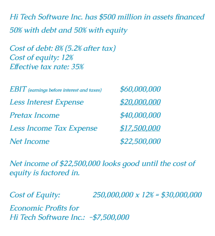
Hi Tech Software Inc. is profitable on an accounting basis, but unprofitable on an Economic Profits basis. The 12% cost of equity is an investor’s required rate of return, also known as the opportunity cost that a company must pay a shareholder to invest in the firm.

Why should investors subtract an amount for the cost of equity? Because if Hi Tech Software Inc. doesn’t deliver the investors’ required rate of return, they can choose another investment. In fact, investors can buy risk-free Treasury securities if the added risk of a given stock investment isn’t appropriately compensated by extra return. Although there is no legal requirement to deliver a return to equity holders (as there is for interest and principal paid to bondholders), firms must compensate for investment risk exposure in order to attract investors.

The Economic Profits Model has the additional benefit of slicing up cash flows to give us insight on whether management’s capital allocation decisions (dividend policy, share repurchase, acquisitions, etc.) create or destroy value over time. It is similar to modern corporate finance theory, whereby management teams strive to take on only projects that have a positive net present value.

A Real World Example

Let’s bridge the gap between the hypothetical and the real world by walking through a calculation of economic profits for technology giant, Oracle Corporation. The following example will take us through the steps of calculating economic profits. The equation for economic profits is as follows:

Economic Profit = Net Operating Profit after Taxes Minus Capital Charges

Step 1: Calculating Net Operating Profit After Taxes (NOPAT)

To calculate NOPAT, start with earnings before interest and taxes (EBIT) on the income statement and subtract the tax liability. Using the sample income statement in Figure 2 below, we calculated Oracle’s NOPAT for the fiscal years 2012, 2013, 2014, 2015 and 2016, as outlined in Figure 3 below.

Figure 2: Oracle Corporation Income Statement

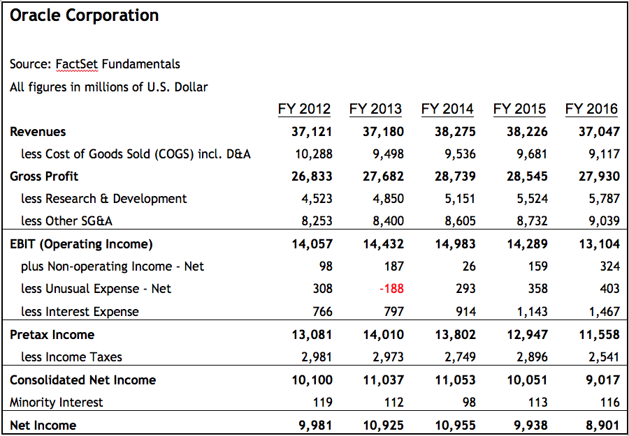
Source: Source: FactSet Fundamentals

Step 2: Calculating Invested Capital

After we determine NOPAT, the next step is to calculate the firm’s total invested capital – all money that has been invested in the company. This money provides the operating assets required for core business activities like inventory, property, plant, and equipment. There are a few different ways to calculate invested capital including the following:

Figure 3: NOPAT Calculation

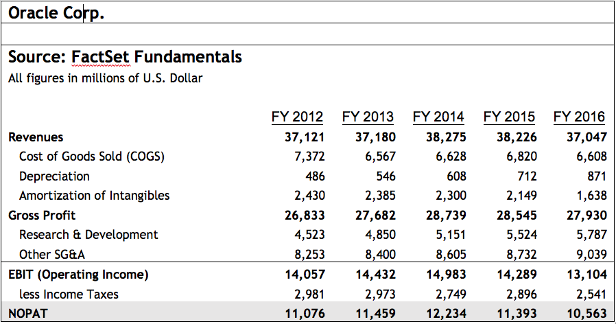
Source: Source: FactSet Fundamentals

Invested Capital

= Book Value of Debt + Book Value of Equity

= Fixed Assets + Current Assets – Current Liabilities – Cash

= Fixed Assets + Non-cash Working Capital

Invested capital is an estimate of the total funds held on behalf of shareholders, lenders, and any other financing sources. A key concept in the calculation of Economic Profits is that a company is charged “rent” for the use of these funds. Economic Profits then represents all profit in excess of this rental charge.

Continuing with the Oracle example, we calculate the firm’s invested capital at the end of 2016 as follows:

Invested Capital = Book Value of Debt + Shareholders’ Equity

= ($3.75 + $40.11) + $47.29 = $91.15

Step 3: Calculating the Cost of Debt

Because interest expense is deductible from income taxes, we define the cost of debt on an after-tax basis as follows:

Cost of Debt = (Interest Expense / Total Debt) * (1- tax rate)

= ($1.467 / ($3.75 + $40.11)) * (1 – 21%) = 2.6%

Figure 4: Oracle Corp. Balance Sheet

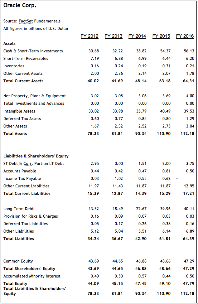
Source: Source: FactSet Fundamentals

Step 4: Calculating the Required Return on Equity

The required return on equity for an investment is the risk-free rate, such as a U.S. Treasury, plus a risk premium equivalent to the same risk as the investment under consideration. If a risk asset has an expected return equivalent to that of a risk-free asset, it would only make sense to buy the risk-free asset and avoid the risk asset.

When evaluating equities for potential investment we are interested in the rate of return an investor would require to hold the equity instead of the risk-free asset. This is referred to as the required return on equity and can be estimated using the Capital Asset Pricing

Model (CAPM).

Required Return on Equity= rf + β (rm – rf)

Where:

rf = the risk-free rate, typically the interest rate of the 10-year US Treasury

β = the trailing 3-year beta for the equity under consideration vs. the S&P 500

rm = the expected market return. A simple way to estimate this is by taking the expected earnings yield of the S&P 500, which is equivalent to the inverse of the price/earnings multiple of that same index

The (rm – rf) term is also known as the equity risk premium. This is the excess return an investor would require to hold equities instead of the risk-free asset. It has historically ranged between 3% and 5%.

Figure 5: Treasury Yields

Assume that we plan to hold an investment for the next 10 years. As of Feb 28, 2017, the forward 12-month P/E for the S&P 500 was 18.11x, which equates to an earnings yield of 5.52%. Another way to think about this is that investors expect the S&P 500 to return approximately 5.52% over the next 12 months. Using this information as well as the data from Figure 5, we can estimate the required rate of return for Oracle using the capital asset pricing model (CAPM) as follows:

Required Return on Equity= rf + β (ERP) = 2.50 + 1.07 (3.02) = 5.73%

Where:

Risk Free Rate (Rf) = 2.50%

Equity Risk Premium (ERP) = rm – rf = 5.52% – 2.5% = 3.02%

Beta (β) for Oracle (3-year trailing vs. S&P 500) = 1.07

Step 5: Calculating the Weighted Average Cost of Capital (WACC)

The weighted average cost of capital (WACC) is the rate of return that could have been earned by putting the same money into a different investment with equal risk. Thus, the WACC is the rate of return required to persuade an investor to make a given investment.

It is helpful to think of this as the investor’s opportunity cost of owning a particular investment. WACC is the rate that should be used to discount future cash flows to a present value. Companies that have well established business models, stable cash flows, manageable leverage, and a competitive edge should have a lower risk factor (β) than the market and thus a lower required rate of return.

Continuing with the Oracle example, we calculate the WACC as follows:

WACC = [(Debt/Total Capitalization)*Cost of Debt] + [(Equity/ Total Capitalization)*Cost of Equity]

= [($43.855 / $91.144) * 2.6%] + [($47.289 / $91.144) * 5.73%] = 4.22%

Step 6: Calculating Economic Profits

As we stated earlier, economic profits equal the firm’s net operating profit after taxes minus a capital charge. The capital charge is calculated by multiplying the total invested capital at the end of the period by the WACC as follows:

Capital Charge = WACC x Invested Capital

Capital Charge = 4.2% x $91,144 = $3,840

Figure 6: Calculating Economic Profits for Oracle Corp.

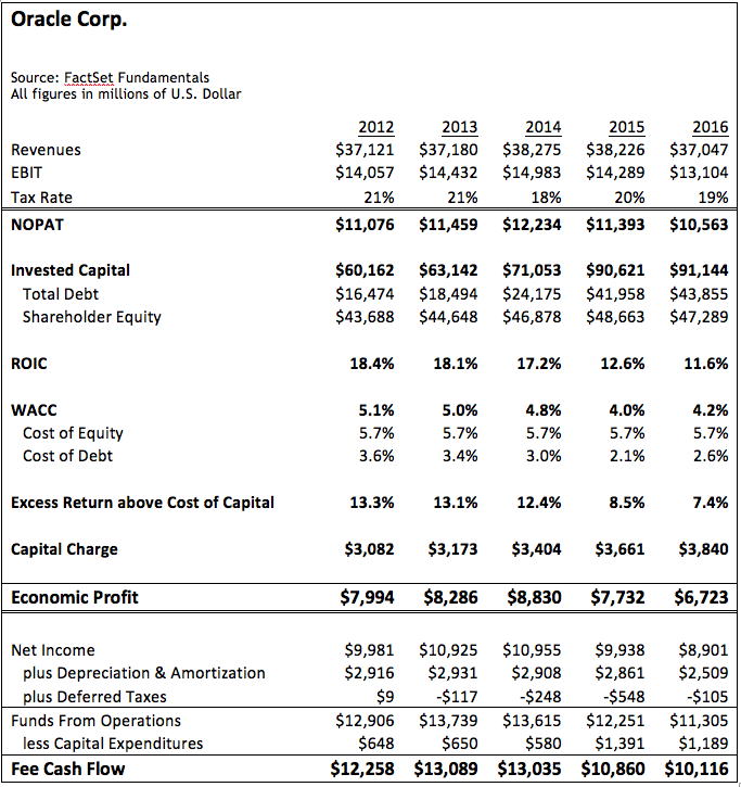
Source: Source: FactSet Fundamentals

Subtracting the capital charge from NOPAT we arrive at a value for economic profits:

Economic Profits = $10,563 – $3,840 = $6,723

Economic Profits for Oracle Corp. for the years 2012 through 2016 are summarized in Figure 6 below.

What can we take away from this example? In short, we see that Oracle created value for its shareholders over the five-year period. Not only did the company generate an impressive $59 billion in cumulative free cash flow, it also created in excess of $39 billion in Economic Profits, as a result of the positive spread between ROIC and WACC. Though this spread has narrowed (from 13.3% to 7.4%) over the last five years, it is still quite impressive. Positive economic profits indicate that management should continue to invest in the business as long as risk and return for future projects is similar to that of previous projects. If it continues to invest, Oracle should continue to generate positive economic profits and thus create wealth for its shareholders.

On the other hand, if economic profits were negative, Oracle management should consider shifting investment from projects with negative economic profits into those with positive economic profits or, if no such projects are identified, the company should return capital to shareholders through stock buybacks or dividend payments. Oracle may also consider acquiring a company or division with higher economic profits than it produces internally, but only if it pays a reasonable price for those assets. The bottom line is – only take actions that result in positive economic profits. If a management action results in negative economic profits, it will ultimately destroy value for shareholders, and the company’s price will decrease.

Let’s consider another example, Valeant Pharmaceuticals (VRX). Using the same methodology as the previous Oracle example, we have calculated the company’s free cash flow and Economic Profits in Figure 6 below. At first glance, it appears that Valeant has created over $4 billion in value for shareholders over the five-year period, based on free cash flow. However, using the Economic Profits Model, we see that Valeant actually destroyed wealth for shareholders in all but one year. In total, the company destroyed over $2.8 billion in shareholder wealth. This example highlights the importance of considering capital structure when choosing investments. Recall that DCF models only subtract the cost of debt by deducting interest expense from operating income. Economic Profits also factor the cost of equity into the equation.

The examples of Oracle Corp. and Valeant Pharmaceuticals show how useful the Economic Profits Model can be in assessing whether management’s prior capital allocation decisions have created or destroyed wealth for shareholders. However, the Economic Profits Model is also useful as a valuation tool to assist in determining a company’s intrinsic value, which can then be used to derive a fair value for the firm’s equity. The Economic Profits Model is the primary valuation tool we employ at QSV Equity Investors.

Economic Profits as a Valuation Tool

Economic Profit is based on the same idea as discounted free cash flow. However, with the Economic Profits Model, the firm’s total value is broken into two parts: invested capital and the present value of future economic profits. The sum of these two parts equals the firm’s intrinsic value. The theory behind economic profits was developed by Bennett Stewart in the 1980s and presented in his best-selling book, The Quest for Value.

Figure 7: Economic Profits for Valeant Pharmaceuticals

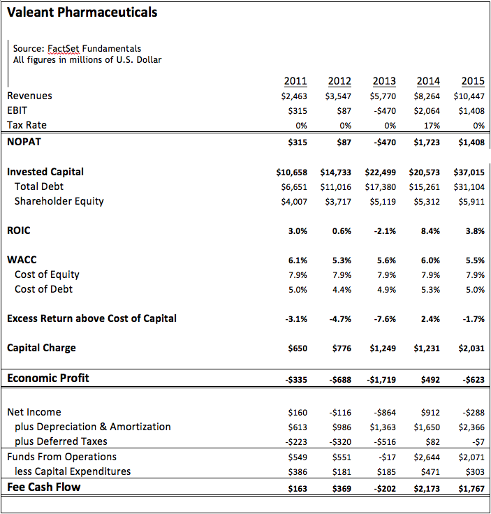
Source: Source: FactSet Fundamentals

Figure 8: Using Economic Profits as a Valuation Tool

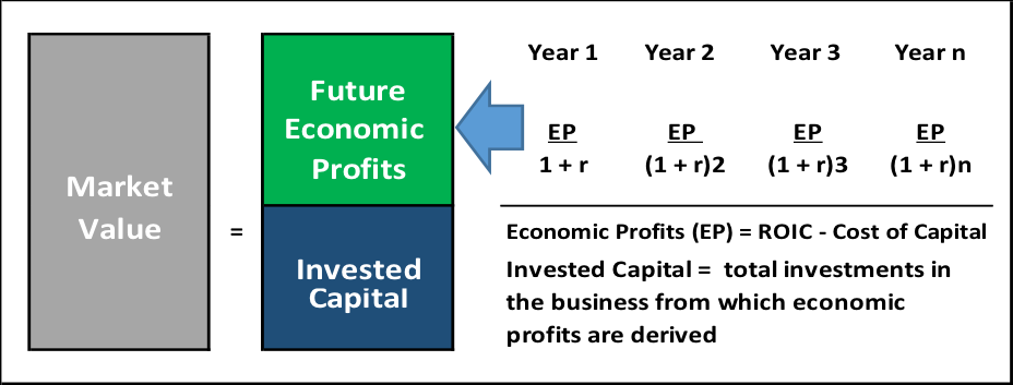
The Value of a Firm = Invested Capital + Present Value of Future Economic Profits

Economic profit is profit after all costs, including the cost of borrowing investors’ funds. If economic profit is increasing, then the firm’s intrinsic value is also increasing, suggesting that market value should

also increase.

Recall that the Economic Profits and Cash Flow Models arrive at the same intrinsic value for a company. However, we believe the Economic Profits Model provides additional insight into whether management’s capital allocation decisions are creating or destroying value, which makes this model a better choice for valuing a firm.

Of course, the limitation on both models is that they are only as good as the data input into the model. In other words, garbage in/garbage out. Both models require successfully forecasting a number of variables in order to arrive at an accurate firm value. Admittedly, this can be more art than science. However, we believe that in the hands of experienced investment professionals the Economic Profits Model can be a powerful tool in determining a company’s intrinsic value.

Let’s continue with our earlier Oracle analysis. This example oversimplifies the process, but still provides a reasonable overview of the methodology. For this example, we have made the following assumptions:

• Revenues are projected to grow at 3% for the first five years and then drop to 2% thereafter.
• EBIT margins start at 35%, consistent with fiscal year 2016, and subsequently decay by 1% per year.
• Tax rate is assumed to be in line with the 10-year average at 25%.
• Total debt is assumed to remain constant.
• For simplicity, WACC is assumed to remain constant at 6%. In reality, this number changes over time as the capital structure changes and interest rates fluctuate.

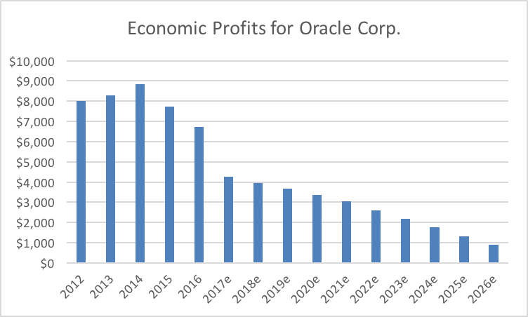
Using the set of assumptions above, we can project Oracle’s economic profits well into the future as shown in Figure 9.

It’s important to note that economic profits peaked in 2014 and, based on the data presented here, are projected to trend down until 2026. This means that Oracle is expected to generate ROIC greater than its cost of capital until 2026 and after that point level off.

Calculating Terminal Value

When building a valuation model, there is a stated forecast period for which analysts make very detailed assumptions about a firm’s future growth and profitability. As investors, we would all like to own companies that grow economic profits at an attractive rate forever, well beyond our forecast period. However, the reality is that most if not all firms eventually settle into a steady state where the spread between ROIC and WACC stabilizes. This does not mean the firm no longer grows, it simply signifies a transition into middle age and maturity. An effective valuation model must account for this transition period.

To account for this transition period beyond the stated forecast period, we rely on concept known as Terminal or Continuing Value. Terminal Value represents future economic profits far into the future, discounted back to the present.

Terminal Value = ((ROIC – WACC) / WACC) / (1+WACC)ⁿ

If we determine that economic profits are positive during the transition period, the terminal value will be positive and add to the intrinsic value of the firm. If economic profits are zero, meaning ROIC = WACC, the terminal value will equal zero and will have no effect on intrinsic value. Lastly, if ROIC is less than WACC, the firm is expected to destroy value and will decrease the current intrinsic value of the firm.

The length of a model’s stated forecast period determines what portion of a firm’s total value is attributable to the Terminal Value. The shorter the stated forecast period, the greater the percentage of total firm value attributable to Terminal Value, and vice versa. Typical forecast periods range from 5 to 20 years. At QSV, we prefer to use a 20-year period. Although it can be more challenging to accurately forecast that far into the future, a 20-year period allows us to adequately factor mean reversion into our models and to taper the ROIC toward the cost of capital over time. A longer period also allows us to vary the competitive advantage period and evaluate multiple growth scenarios. To simplify the Oracle Corp. example, we shortened the stated forecast period to 10 years. Beyond that forecast period, Oracle still generates profits. Terminal Value is how we estimate what these future undetermined profits are worth.

The most commonly used method of establishing a Terminal or Continuing Value is to assume that the Economic Profits generated in the final year of

Figure 9: Economic Profit Valuation for Oracle Corp.

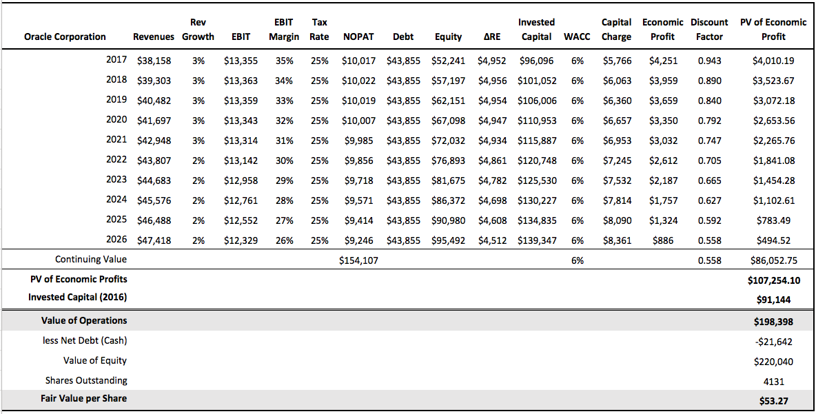
Figure 10: Economic Profits

the stated forecast period remain constant going forward. Those Economic Profits are then divided by the final year WACC to arrive at a Terminal Value for the company. This is a very conservative method of estimating Terminal Value, and in many cases, understates a company’s value. However, because we are using a 20-year forecast period and because we build a significant amount of mean reversion into our models, we are comfortable that our approach reasonably reflects the middle-age or mature years that lie ahead for the company. To continue with the Oracle example, we calculate a terminal value of $154,107 ($9,246/6%) for the company.

The Final Step: Intrinsic Value

At this point in our stock evaluation process, we have calculated a series of values for an individual company: future Economic Profits for the stated forecast period and a Terminal Value for the company beyond that period. In order to use this information to determine the company’s current value, we take the present value of each of these cash flows by discounting at the WACC as shown above in Figure 9. Adding together the discounted values of each stream of cash flows gives us the present value of future Economic Profits.

In the Oracle example above, the present value of Economic Profits equals $107,254 ($21,202 + $86,052).

There is one final step in determining a company’s intrinsic value. Recall that a company’s fair value is equal to the sum of its total invested capital plus the present value of future economic profits. Returning to the Oracle example, we must therefore add the current year invested capital ($91,144) to the present value of future Economic Profits ($107,254).

This yields an intrinsic value of $198,398 billion for Oracle Corp., which is the dollar amount a potential buyer should be willing to pay for the entire company.

Total Invested Capital + PV of Future Economic Profits = Intrinsic

or Fair Value

$91,144 + $107,254 = $198,398 billion

As equity investors, we want to know how this translates to a fair value for an individual share. Therefore, we subtract the net debt and divide that value by the number of outstanding shares. In the case of Oracle, we would estimate the fair value to be around $53 per share as follows:

Fair Price per Share = (Intrinsic Value – Net Debt) / Shares

Outstanding

= ($198,398 – (-$21,642)) / 4131 = $53

Since the stock’s intrinsic value is $53, investors should consider buying the stock when it trades for less than $53 and selling or shorting it when it trades above $53.

Conclusion

Based on years of investing experience and our understanding of common investor behaviors, we believe there are two primary hurdles that prevent people from being successful investors. The first is the inability to separate day-to-day stock price gyrations from underlying company fundamentals and the second is the tendency to buy stocks when they are priced above value, have returns that are reverting to the mean, and carry higher risk than expected. Conversely, thinking like business owners rather than a stock investors and owning stocks when they are trading below their intrinsic value are two notable advantages for investors.

At QSV, we purposefully act like business owners, focusing on a company’s intrinsic value and blocking out day-to-day price moves. Our stock selection process uses a variety of valuation measures to screen for potential investment opportunities. We then rely on an Economic Profits Model to determine whether a company is able to create wealth, what the company will be worth well into the future and what is a fair price for the company in the present. That is how we decide whether or not we want to own a stock. We believe the Economic Profits Model is a powerful tool for choosing stocks that will help our clients beat inflation and create long-term wealth.

Bibliography Stewart, G. Bennett. The quest for value. Harper Collins, 1991.